This lab implements a discrete Bayes filter over a 3D grid of robot states $(x, y, \theta)$, runs it on a recorded simulation trajectory, and compares the estimated pose against the ground truth.
Alogrithm
Each cell stores the belief $bel(x_t) = p(x_t \mid z_{1:t}, u_{1:t})$ — the posterior over the robot pose conditioned on all past readings. Under the Markov assumption (Lec. 17), the filter alternates two steps:
$$\overline{bel}(x_t) = \sum_{x_{t-1}} p(x_t \mid u_t, x_{t-1}), bel(x_{t-1}) \quad \text{(Prediction)}$$
$$bel(x_t) = \eta , p(z_t \mid x_t) , \overline{bel}(x_t) \quad \text{(Update)}$$
Prediction propagates the belief through the motion model (uncertainty grows); update multiplies in the sensor likelihood (uncertainty shrinks). $\eta$ normalizes the belief to sum to 1.
Compute Control
The odometry model (Lec. 18) decomposes relative motion into an initial rotation, a translation, and a final rotation:
$$\delta_{rot1} = \mathrm{atan2}(y_{cur} - y_{prev},, x_{cur} - x_{prev}) - \theta_{prev}$$
$$\delta_{trans} = \sqrt{(x_{cur} - x_{prev})^2 + (y_{cur} - y_{prev})^2}$$
$$\delta_{rot2} = \theta_{cur} - \theta_{prev} - \delta_{rot1}$$
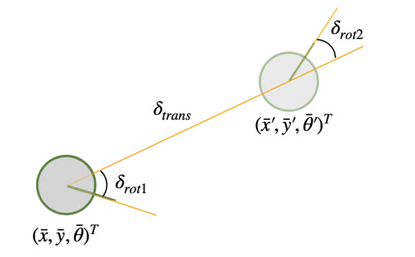
I broadcast the poses with numpy so the same function handles a single pair or the full grid in one call. Translations below $10^{-4}$ m are treated as pure rotations to avoid atan2 instability, and angles wrap to $[-180^\circ, 180^\circ]$.
def compute_control(cur_pose, prev_pose):
    """ Given the current and previous odometry poses, this function extracts
    the control information based on the odometry motion model.

    Args:
        cur_pose  ([Pose]): Current Pose
        prev_pose ([Pose]): Previous Pose

    Returns:
        [delta_rot_1]: Rotation 1  (degrees)
        [delta_trans]: Translation (meters)
        [delta_rot_2]: Rotation 2  (degrees)
    """

    # Convert to numpy arrays
    cur_pose = np.array(cur_pose)
    prev_pose = np.array(prev_pose)
    x_prev, y_prev, yaw_prev = prev_pose[..., 0], prev_pose[..., 1], prev_pose[..., 2]
    x_cur,  y_cur,  yaw_cur  = cur_pose[..., 0],  cur_pose[..., 1],  cur_pose[..., 2]
    x_cur, x_prev = np.broadcast_arrays(x_cur, x_prev)
    y_cur, y_prev = np.broadcast_arrays(y_cur, y_prev)
    yaw_cur, yaw_prev = np.broadcast_arrays(yaw_cur, yaw_prev)

    # 1. Translation
    dx = x_cur - x_prev
    dy = y_cur - y_prev
    delta_trans = np.hypot(dx, dy)

    # If translation is  small, treat it as a pure rotation
    mask = delta_trans >= 1e-4

    # 2. Rotation 1
    delta_rot_1 = np.zeros_like(delta_trans)
    delta_rot_1[mask] = np.degrees(np.arctan2(dy[mask], dx[mask])) - yaw_prev[mask]
    delta_rot_1 = norm_angle(delta_rot_1)

    # 3. Rotation 2
    delta_rot_2 = np.zeros_like(delta_trans)
    delta_rot_2[mask] = yaw_cur[mask] - yaw_prev[mask] - delta_rot_1[mask]
    delta_rot_2[~mask] = yaw_cur[~mask] - yaw_prev[~mask]
    delta_rot_2 = norm_angle(delta_rot_2)

    return np.squeeze(delta_rot_1), np.squeeze(delta_trans), np.squeeze(delta_rot_2)
Odometry Motion Model
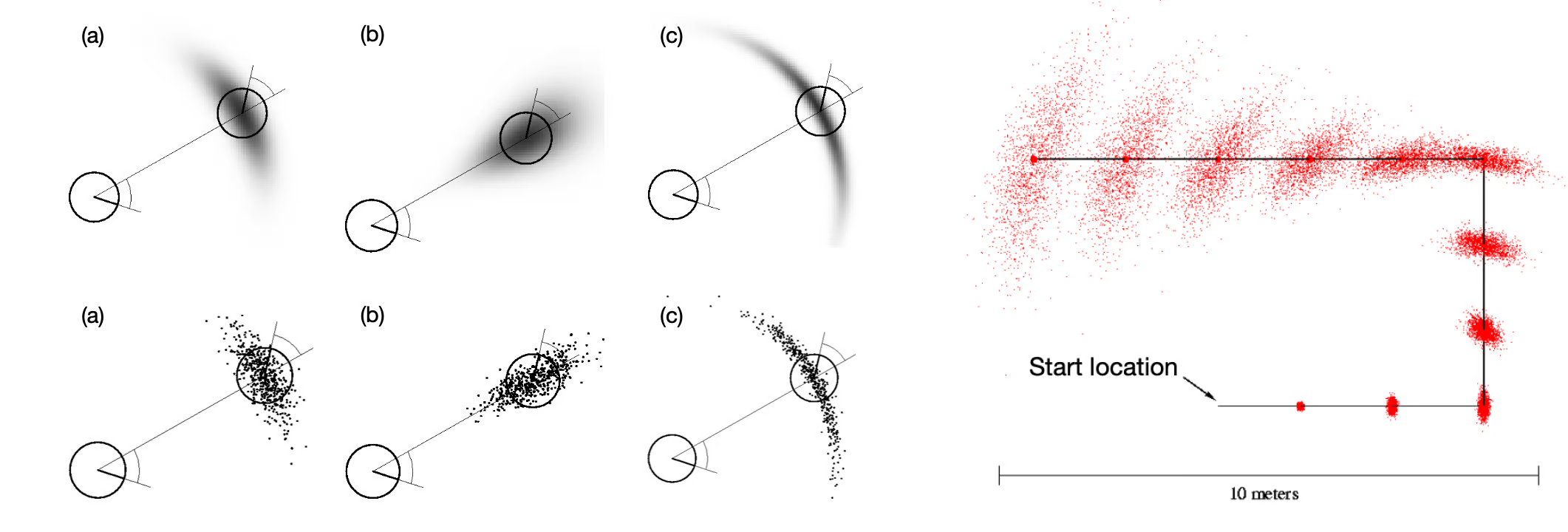
The motion model returns $p(x_t \mid u_t, x_{t-1})$. I run compute_control on the candidate poses $x_{t-1}, x_t$ to get the expected control, subtract from the reported $u_t$ to obtain three errors $e_{rot1}, e_{trans}, e_{rot2}$, and evaluate each under an independent zero-mean Gaussian:
$$p(x_t \mid u_t, x_{t-1}) = \mathcal{N}(e_{rot1};, 0, \sigma_{rot}^2) \cdot \mathcal{N}(e_{trans};, 0, \sigma_{trans}^2) \cdot \mathcal{N}(e_{rot2};, 0, \sigma_{rot}^2)$$
$\sigma_{rot}$ and $\sigma_{trans}$ (from world.yaml) control how noisy the motion model is.
def odom_motion_model(cur_pose, prev_pose, u):
    """ Odometry Motion Model

    Args:
        cur_pose  ([Pose]): Current Pose
        prev_pose ([Pose]): Previous Pose
        (rot1, trans, rot2) (float, float, float): A tuple with control data in the format
                                                   format (rot1, trans, rot2) with units (degrees, meters, degrees)


    Returns:
        prob [float]: Probability p(x'|x, u)
    """
    rot1_u, trans_u, rot2_u = u
    rot1_exp, trans_exp, rot2_exp = compute_control(cur_pose, prev_pose)

    # Compute Errors
    err_rot1 = norm_angle(rot1_u - rot1_exp)
    err_trans = trans_u - trans_exp
    err_rot2 = norm_angle(rot2_u - rot2_exp)

    # Compute Gaussian Probabilities
    p1 = loc.gaussian(err_rot1, 0.0, loc.odom_rot_sigma)
    p2 = loc.gaussian(err_trans, 0.0, loc.odom_trans_sigma)
    p3 = loc.gaussian(err_rot2, 0.0, loc.odom_rot_sigma)

    # Combine probabilities (assuming independence)
    prob = p1 * p2 * p3
    return prob
Prediction Step
The grid is $12 \times 9 \times 18 = 1944$ cells, so a naive double loop needs $1944^2 \approx 3.8$ M transitions per step. Two optimizations:
- Skip negligible cells. Only previous cells with $bel(x_{t-1}) > 10^{-4}$ contribute. After a few updates the belief is peaked, so this is usually a handful of cells.
- Vectorize over current poses. Build the full $1944 \times 3$ array of candidate $x_t$ once and pass it to
odom_motion_model— every previous cell then yields a full slab in one numpy call.
Finally I normalize $\overline{bel}$ to prevent underflow when many small Gaussians multiply.
def prediction_step(cur_odom, prev_odom):
    """ Prediction step of the Bayes Filter.
    Update the probabilities in loc.bel_bar based on loc.bel from the previous time step and the odometry motion model.

    Args:
        cur_odom  ([Pose]): Current Pose
        prev_odom ([Pose]): Previous Pose
    """
    u = compute_control(cur_odom, prev_odom)
    loc.bel_bar = np.zeros_like(loc.bel)

    all_x = loc.mapper.x_values.flatten()
    all_y = loc.mapper.y_values.flatten()
    all_a = loc.mapper.a_values.flatten()
    all_cur_poses = np.column_stack((all_x, all_y, all_a))


    # Skip cells with negligible belief
    valid_prev_indices = np.argwhere(loc.bel > 0.0001)

    # Iterate all possible prev poses with non-negligible belief
    for idx in valid_prev_indices:
        # Get previous pose and its belief
        cx, cy, ca = idx
        prev_prob = loc.bel[cx, cy, ca]
        x_prev, y_prev, a_prev = loc.mapper.from_map(cx, cy, ca)
        prev_pose = np.array([x_prev, y_prev, a_prev])

        # Compute transition probabilities for all current poses
        prob_transition = odom_motion_model(all_cur_poses, prev_pose, u)
        loc.bel_bar += prob_transition.reshape(loc.bel_bar.shape) * prev_prob

    # Normalize to prevent arithmetic underflow
    bel_bar_sum = np.sum(loc.bel_bar)
    if bel_bar_sum > 0:
        loc.bel_bar /= bel_bar_sum
Sensor Model
The 18 rays are treated as conditionally independent given $x_t$ and the map (Lec. 19):
$$p(z_t \mid x_t) = \prod_{k=1}^{K=18} p(z_t^k \mid x_t, m)$$
For each ray I use a Gaussian around the ray-cast expected reading $z_t^{k*}$ — the likelihood-field model from Lec. 19 with $p_{max}$ and $p_{rand}$ folded into a single $\sigma_{sensor}$:
$$p(z_t^k \mid x_t, m) = \mathcal{N}(z_t^k - z_t^{k*};, 0, \sigma_{sensor}^2)$$
sensor_model(obs) returns the per-ray likelihood vector. The expected scans are pre-computed in loc.mapper.obs_views, so no ray casting happens at runtime.
def sensor_model(obs):
    """ This is the equivalent of p(z|x).


    Args:
        obs ([ndarray]): A 1D array consisting of the true observations for a specific robot pose in the map

    Returns:
        [ndarray]: Returns a 1D array of size 18 (=loc.OBS_PER_CELL) with the likelihoods of each individual sensor measurement
    """
    error = loc.obs_range_data - obs
    prob_array = loc.gaussian(error, 0.0, loc.sensor_sigma)
    return prob_array
Update Step
Multiply $\overline{bel}$ pointwise by the per-cell sensor likelihood and renormalize:
$$bel(x_t) = \eta , p(z_t \mid x_t) , \overline{bel}(x_t), \quad \eta = \left(\sum_{x_t} p(z_t \mid x_t),\overline{bel}(x_t)\right)^{-1}$$
Fully vectorized: actual_obs - expected_obs broadcasts over the $(12,9,18,18)$ tensor, and np.prod(..., axis=-1) collapses the 18 rays into one likelihood per cell. If $\sum bel$ underflows I fall back to $bel = \overline{bel}$.
def update_step():
    """ Update step of the Bayes Filter.
    Update the probabilities in loc.bel based on loc.bel_bar and the sensor model.
    """
    # Compute the expected observations & their probabilities
    actual_obs = loc.obs_range_data.flatten().reshape(1, 1, 1, -1)
    expected_obs = loc.mapper.obs_views
    likelihoods = loc.gaussian(actual_obs - expected_obs, 0.0, loc.sensor_sigma)

    # Compute Naive Likelihood p(z|x)
    p_z_given_x = np.prod(likelihoods, axis=-1)

    # Bayesian Update: Prior * Naive Likelihood = Posterior
    loc.bel =  p_z_given_x *loc.bel_bar

    # Normalize to prevent arithmetic underflow
    bel_sum = np.sum(loc.bel)
    if bel_sum > 0:
        loc.bel /= bel_sum
    else:
        loc.bel = loc.bel_bar
Simulation
The simulator splits into a robot display that draws the robot inside the virtual world and a plotter that overlays the belief against ground truth, connected through the Commander. Each step the robot does $\delta_{rot1} \to \delta_{trans} \to \delta_{rot2}$, then spins in place to collect the 18-ray scan that drives the update. Three trajectories are plotted: ground truth (green), pure odometry (red), and the Bayes-filter belief over the most-probable cell (blue).
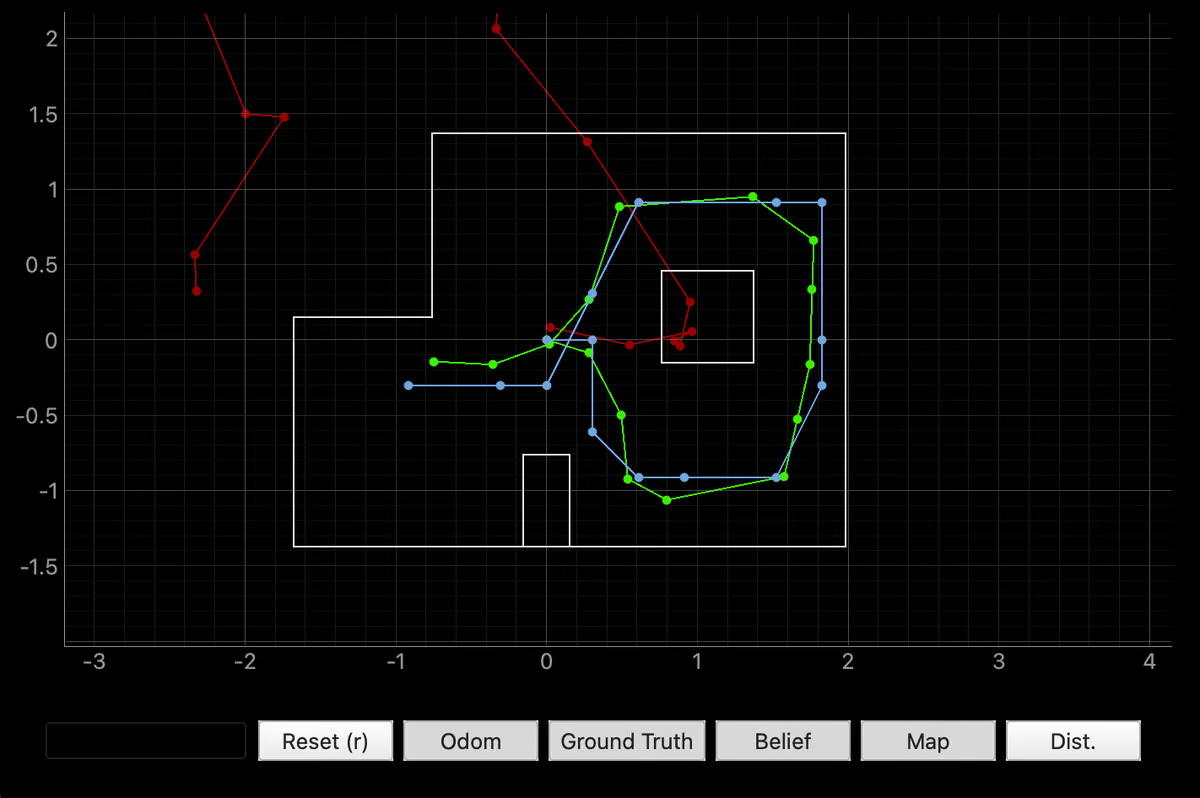
Blue tracks green closely throughout the run, while red drifts off the map after a few steps because odometry errors accumulate without sensor correction — exactly the predicted behavior. A few limitations are visible:
- Discretization. The belief is pinned to cell centers ($0.3048$ m, $20^\circ$), so the blue line can only snap to the closest cell rather than follow green exactly.
- Feature-poor regions. Along the rightmost hallway, most rays hit the same two parallel walls, so neighboring cells produce nearly identical expected scans and the filter cannot disambiguate along the hallway axis until a corner is reached.
- Limited ray angles. 18 rays over 360° leave thin gaps that can fall between consecutive rays.
Overall the trace confirms the prediction step, sensor model, and update step are all working: the filter recovers the true pose after each measurement and never diverges, even from a uniform prior.