This lab extended the localization framework from simulation to the physical robot. While Lab 10 used both the prediction and update steps of the Bayes filter, this lab focused only on the update step using full 360-degree ToF sensor scans. I focused on how localization performance changes when moving to a real-world system with sensor noise, imperfect rotation, and hardware limitations.
Simulation
Before moving to the real robot, I verified the Bayes filter implementation from Lab 10 by running lab11_sim.ipynb. This notebook executes a pre-recorded trajectory and overlays three trajectories: the ground truth (green), the raw odometry estimate (red), and the belief from the Bayes filter (blue).
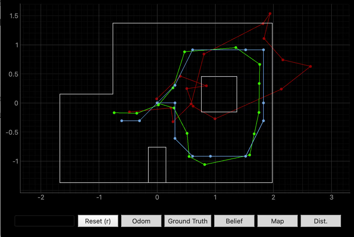
The blue line is almost identical to the result I obtained in Lab 10 and tracks the ground truth closely throughout the trajectory. In contrast, the red odometry-only line drifts substantially from the ground truth and accumulates error over time, especially after multiple rotations. This confirms that my Lab 10 implementation of the prediction step, the sensor model, and the update step are still working correctly, and that the Bayes filter is significantly more reliable than dead reckoning on noisy motion data.
Algorithm
On the real robot, only the update step of the Bayes filter is executed: the robot stands still at a marked pose, performs an in-place 360° rotation, and uses 18 equally-spaced ToF readings (one every 20°) as the observation vector. The prediction step is skipped, so the prior bel_bar is set to a uniform distribution before each update.
I reused the orientation-PID mapping FSM (MAP_START → MAP_TURN → MAP_STABILIZE → MAP_MEASURE → MAP_DONE) from Lab 9 directly, since it already provides accurate 20° increments with low rotational drift. The only modifications on the Arduino side were the BLE commands sent from perform_observation_loop: SET_MAP_DEGREES = 360, SET_MODE = 5, the orientation PID gains $K_p = 2.5, K_i = 1.2, K_d = 0.25$ from Lab 6, and the sample/duration parameters needed to complete a full rotation.
On the Python side, the observation loop is implemented as an async function so it can be awaited inside the localization framework (await loc.get_observation_data() internally calls asyncio.run on this coroutine). The flow is:
- Clear all internal buffers (
times,yaws,tof_1_readings,tof_2_readings). - Send BLE commands to start the 360° mapping turn and
await asyncio.sleep(25)to let the rotation finish. - Subscribe to the
RX_STRINGcharacteristic, issueSEND_LOG, and wait for all logged samples to arrive. - Unwrap the IMU yaw with
np.unwrap, filter invalid ToF readings (≤ 0 or ≥ 6000 mm), apply the 69.85 mm sensor offset from Lab 9, and convert from mm to meters. - Return the first 18 valid samples as a column vector with
np.array(ranges_in_meters)[np.newaxis].T, which is the shape the localization module expects.
from notebooks import ble

class RealRobot():
    """A class to interact with the real robot
    """
    def __init__(self, commander, ble):
        # Load world config
        self.world_config = os.path.join(str(pathlib.Path(os.getcwd()).parent), "config", "world.yaml")

        self.config_params = load_config_params(self.world_config)

        # Commander to commuincate with the Plotter process
        # Used by the Localization module to plot odom and belief
        self.cmdr = commander

        # ArtemisBLEController to communicate with the Robot
        self.ble = ble
        self.times = []
        self.yaws = []
        self.tof_1_readings = []
        self.tof_2_readings = []

    def log_handler(self, sender, data: bytearray):
        parts = self.ble.bytearray_to_string(data).split("|")
        if len(parts) == 4:
            timestamp = float(parts[0][2:])
            yaw = float(parts[1][3:])
            tof_1 = float(parts[2][3:])
            tof_2 = float(parts[3][3:])
            self.times.append(float(timestamp))
            self.yaws.append(float(yaw))
            self.tof_1_readings.append(float(tof_1))
            self.tof_2_readings.append(float(tof_2))
            print (f"Received log: timestamp={timestamp}, yaw={yaw}, tof_1={tof_1}, tof_2={tof_2}")

    async def perform_observation_loop(self, rot_vel=120):
        """Perform the observation loop behavior on the real robot, where the robot does
        a 360 degree turn in place while collecting equidistant (in the angular space) sensor
        readings, with the first sensor reading taken at the robot's current heading.
        The number of sensor readings depends on "observations_count"(=18) defined in world.yaml.

        Keyword arguments:
            rot_vel -- (Optional) Angular Velocity for loop (degrees/second)
                        Do not remove this parameter from the function definition, even if you don't use it.
        Returns:
            sensor_ranges   -- A column numpy array of the range values (meters)
            sensor_bearings -- A column numpy array of the bearings at which the sensor readings were taken (degrees)
                               The bearing values are not used in the Localization module, so you may return a empty numpy array
        """
        _ = rot_vel
        # 1. Clear previous readings
        self.times = []
        self.yaws = []
        self.tof_1_readings = []
        self.tof_2_readings = []

        # 2. Send commands to configure the 360 degree rotation, set mode, and start
        observations_count = self.config_params["mapper"]["observations_count"]
        # self.ble.send_command(CMD.SET_MAP_COUNT, str(observations_count))
        self.ble.send_command(CMD.SET_MAP_DEGREES, "360")

        self.ble.send_command(CMD.SET_MODE, "5")
        self.ble.send_command(CMD.UPDATE_ORIENT_PID, "2.5|1.2|0.25")
        self.ble.send_command(CMD.SET_SAMPLE_RATE, "50")
        self.ble.send_command(CMD.SET_DURATION, "25000")
        self.ble.send_command(CMD.START_RECORD, "")

        await asyncio.sleep(25)

        # 3. Collect sensor readings until the loop is done
        self.ble.start_notify(self.ble.uuid['RX_STRING'], self.log_handler)
        await asyncio.sleep(3)
        self.ble.send_command(CMD.SEND_LOG, "")
        await asyncio.sleep(50)
        self.ble.stop_notify(self.ble.uuid['RX_STRING'])

        # 4. Format the output
        tof_2 = np.array(self.tof_2_readings)
        yaw_unwrapped = np.degrees(np.unwrap(np.radians(self.yaws)))
        yaw_continuous = yaw_unwrapped - yaw_unwrapped[0]

        valid_indices_2 = (tof_2 > 0) & (tof_2 < 6000)
        valid_angles_2 = np.radians(yaw_continuous[valid_indices_2])
        valid_distances_2 = tof_2[valid_indices_2] + 69.85


        if len(valid_distances_2) < observations_count:
            raise RuntimeError(
                f"Insufficient observation samples: tof={len(valid_distances_2)}, expected={observations_count}"
            )

        ranges_in_meters = [reading / 1000.0 for reading in valid_distances_2[:observations_count]]
        sensor_ranges = np.array(ranges_in_meters)[np.newaxis].T
        sensor_bearings = np.array(valid_angles_2[:observations_count])[np.newaxis].T

        print(f"Sensor Ranges (m): {sensor_ranges.flatten()}")
        print(f"Sensor Bearings (rad): {sensor_bearings.flatten()}")

        return sensor_ranges, sensor_bearings
I also revised the noise parameters in world.yaml based on the calibration from Lab 7. The default sensor_sigma = 0.1 m is too loose for our hardware: in Lab 7 I measured a ToF measurement standard deviation of ~16 mm at short range, so I tightened sensor_sigma accordingly. This makes the likelihood function more selective and gives the update step a sharper posterior in cells whose expected scan matches the measurement.
Testing
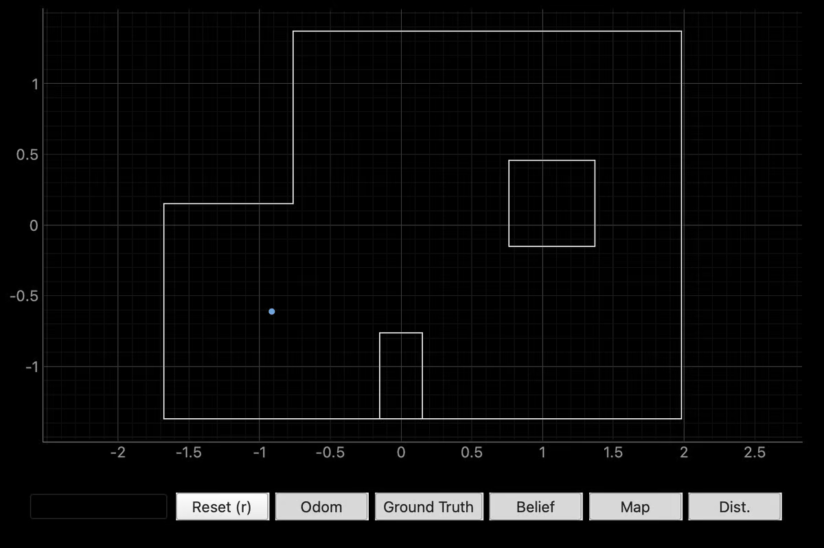
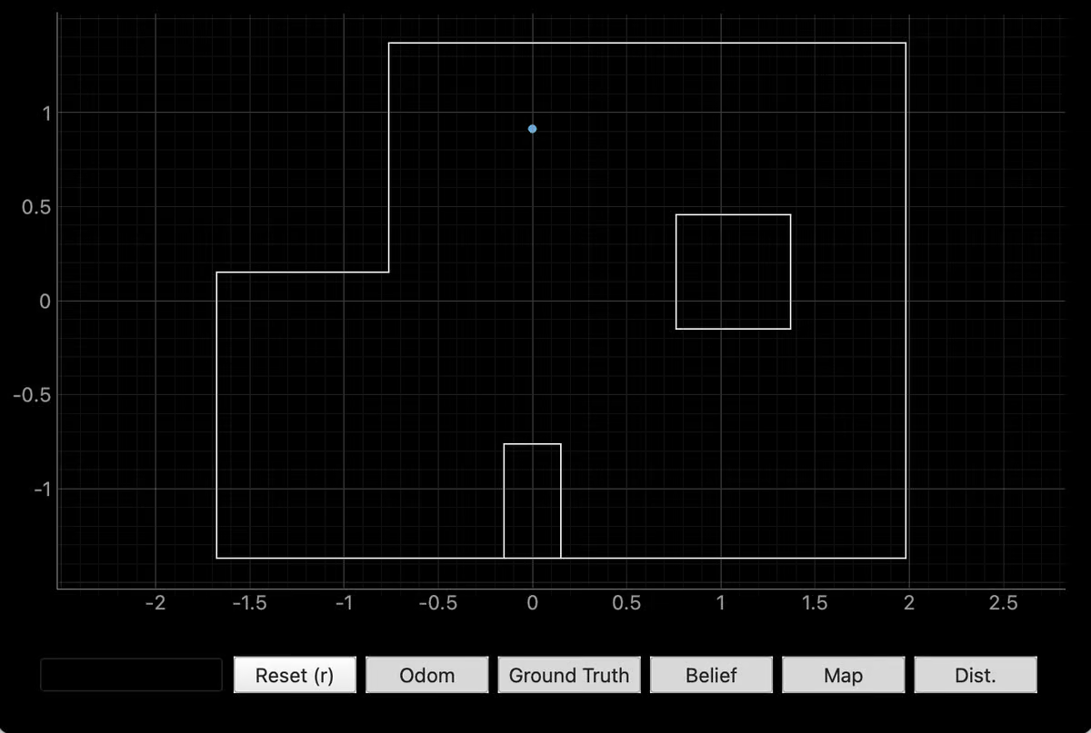
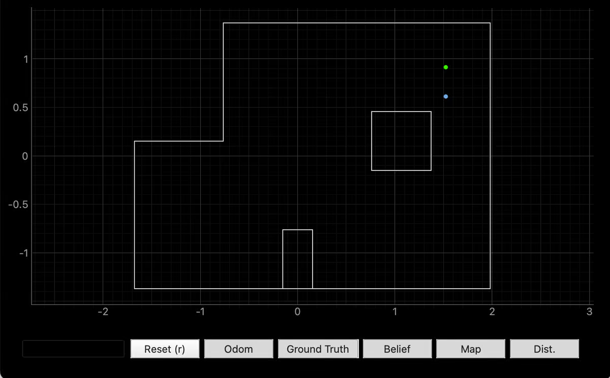
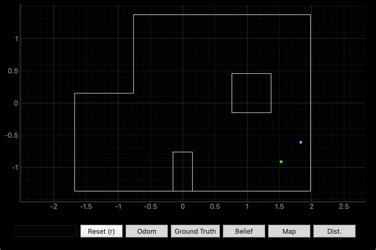
I tested the localization update step at the four marked poses used in Lab 9: $(-3,-2)$, $(0,3)$, $(5,3)$, and $(5,-3)$, all expressed in 1-foot grid units (cell size = 0.3048 m). At each pose, the robot performed one 360° scan and the Bayes filter update produced the belief shown as the blue dot, while the ground truth pose is the green dot.
Pose at (-3,-2)
The belief converged to $(-3,-2)$, matching the ground truth exactly.
Pose at (0,3)
The belief converged to $(0,3)$, again matching the ground truth exactly.
Pose at (5,3)
The belief converged to $(4,3)$, off by one cell (~0.3 m) along the x-axis.
Pose at (5,-3)
The belief converged to $(6,-2)$, off by one cell along both axes.
Analysis
To make the localization results easier to interpret, I also repeated the mapping process from Lab 9 using the same scans collected during the localization runs. The resulting merged map is shown below.
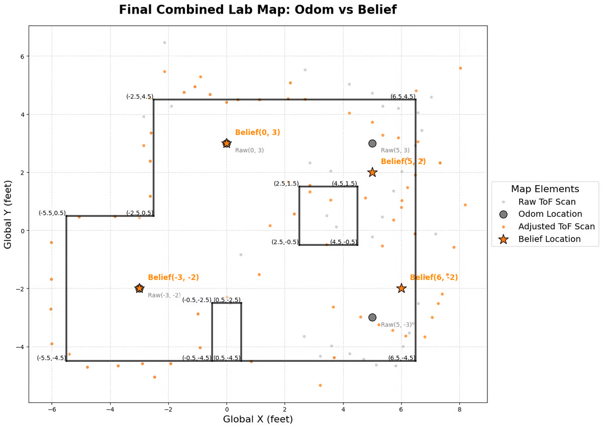
Looking across the four poses, the localization quality clearly correlates with the surrounding map geometry:
-
$(-3,-2)$ and $(0,3)$: accurate. These two poses sit close to multiple walls and to the internal box obstacle, so the 18 scan rays hit a rich set of distinct features at relatively short range. Since the ToF error stays around 30 mm below 2 m (from the Lab 3 calibration), the measured ranges are reliable and the sensor model assigns a sharply peaked likelihood at the correct cell.
-
$(5,3)$ and $(5,-3)$: off by one cell. These poses are far from the internal obstacle and many of the rays must travel across the room to hit the opposite wall. Since there are fewer distinct geometric features nearby to disambiguate the pose, so several neighboring cells produce similar expected scans. And once the ray length exceeds roughly 2 m, the ToF error grows to ~200 mm, which is on the order of a single grid cell. So the posterior spreads across a few adjacent cells and aligns with a neighbouring pose.
To improve performance in these feature-poor regions, I may work on the followings:
- Denser angular sampling: collect more readings per scan (e.g. 36 samples at 10° spacing instead of 18 at 20°) so the likelihood is computed over more independent rays. This would reduce the noise effect of individual ray by averaging out, especially at long range.
- Multiple ToF sensors: my robot already carries two ToF sensors (front and side) and setup in Lab9. Using both during the rotation would double the angular resolution for the same scan time.