In this lab, I integrated an inertial measurement unit (IMU) sensor into the autonomous robot platform I previously built, using the SparkFun RedBoard Artemis Nano microcontroller. The goal is to sense the robot's motion and orientation in real time. Signal processing techniques were applied to achieve reliable state estimation.

Setup IMU

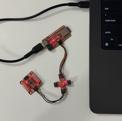
First, I set up the sensor and established communication between it and the board using the I2C interface. Then, I connected the one-to-three port QWIIC connector to the processor and IMU using the braided I2C QWIIC cable. This cable connects VCC, GND, SDA, and SCL to the corresponding microcontroller pins.

For the software, I installed the SparkFun 9DOF IMU Breakout ICM 20948 Arduino Library from the Arduino Library Manager.

Finally, I ran the Example1_Basics test program to verify that the board could successfully initialize the sensor and read the accelerometer and gyroscope values.

Video Here

The sensor generates values based on the right hand rule. The accelerater provided linear acceleration along the x, y, and z axes. When I placed the sensor on the table in stationar, both acceleration on the x and y axes ranged around 0, while the magnitude on z axis was approximately 1 g. When we rotate it on x and y axes, the gravity changes. So, we can use it to estimate the gravity vector and compute static orientation (pitch and roll). However, there are spikes during rapid movement, aking the raw values less reliable for direct angle estimation.

The gyroscope measured angular velocity, responding smoothly to rotations. When I placed the sensor on the table, all three components read 0. As I rotated the board, the values increased.

The AD0_VAL parameter indicates the value of the last bit of the I2C address.On the SparkFun 9DoF IMU breakout, this bit depends on the state of the ADR jumper. When the jumper is open, the pin is pulled high and the address bit equals 1; when the jumper is closed, the bit becomes 0. In this case, we select one to match the hardware configuration..

I will also add a visual indicator to show that the board is running and collecting data for later use in the lab. The LED will blink three times slowly when the board starts up. It will also turn on every time the START_COLLECT_DATA command is called and turn off when the host stops collecting data and requests it.

Accelerometer

To embed the IMU sensor into the board, I included its initialization in the setup() function and added global arrays to store the data.

In the main loop, I incorporated sensor updates, data collection, and calculations. Given a sample ratio, the loop checked and recorded the IMU data as follows:

void
loop()
{
    BLEDevice central = BLE.central();
    if (central) {
        while (central.connected()) {
            write_data();
            read_data();

            if (collecting && sample_count < SAMPLE_LEN) {
                unsigned long current_sample_time = micros();
                if (current_sample_time - last_sample_time >= SAMPLE_INTERVAL) {
                    if (myICM.dataReady()){

                        myICM.getAGMT();

                        raw_acc_x[sample_count] = myICM.accX();
                        raw_acc_y[sample_count] = myICM.accY();
                        raw_acc_z[sample_count] = myICM.accZ();

                        raw_acc_roll[sample_count] = atan2(myICM.accY(), myICM.accZ()) * 180.0 / M_PI;
                        raw_acc_pitch[sample_count] = atan2(myICM.accX(), myICM.accZ())* 180.0 / M_PI;

                        sample_count++;
                        last_sample_time = current_sample_time;
                    }
                }

            }
        }
    }
}

I used the following equations to convert the accelerometer data into pitch and roll:

$\theta = \arctan2 (a_x,a_z)\quad$ $\phi = \arctan2 (a_y,a_z)$

where $\arctan2$ returns $[-\pi, \pi]$

Besides, GET_ACCL_READINGS command is implemented to collect time-stamped accelerometer data and send to the host.

case GET_ACCL_READINGS:
    collecting = false;
    digitalWrite(LED_BUILTIN, LOW);

    for (int i = 0; i < sample_count; i++) {
        tx_estring_value.clear();
        tx_estring_value.append("T: ");
        tx_estring_value.append((int)time_buffer[i]);
        tx_estring_value.append("|p: ");
        tx_estring_value.append(raw_acc_pitch[i]);
        tx_estring_value.append("|r: ");
        tx_estring_value.append(raw_acc_roll[i]);
        tx_characteristic_string.writeValue(tx_estring_value.c_str());
    }

Accuracy Discussion

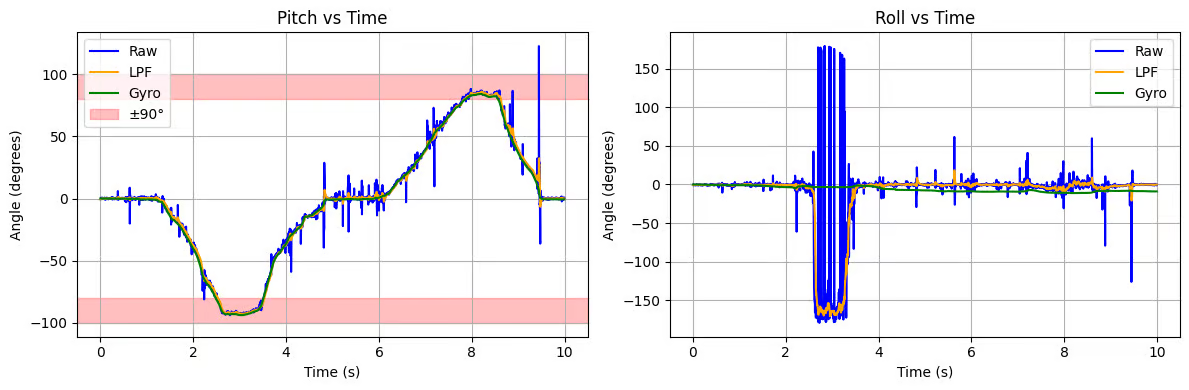
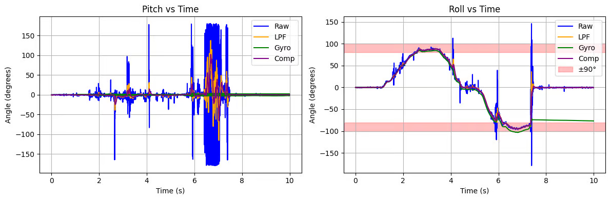
This graph shows the output at pitch rotations of -90, 0, and 90 degrees about the roll axis.

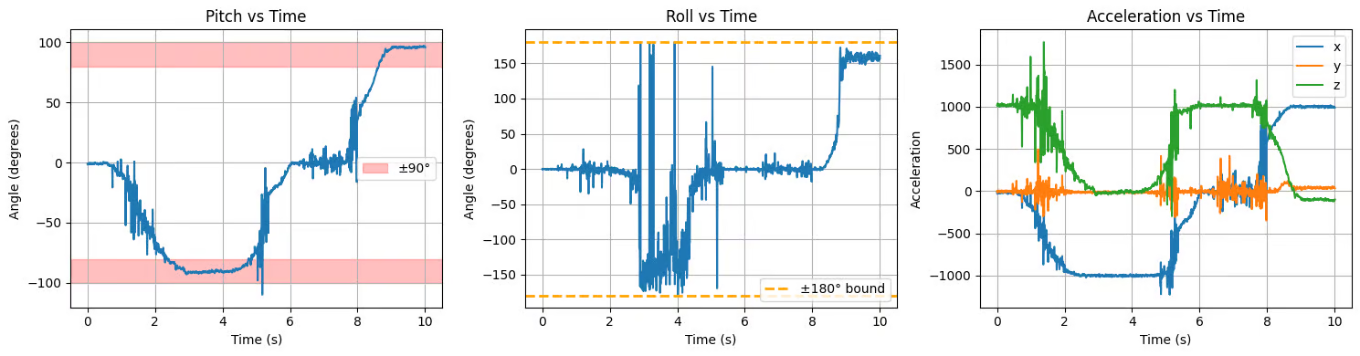
Here, the pitch angle smoothly transitions between target angles and remains relatively stable when stationary. However, short spikes and oscillations appear during motion. At large tilt angles, especially, the roll estimate exhibits significant fluctuations and occasionally approaches the ±180° bound.

The acceleration plots confirm the shift of gravity between components during rotation. For example, the z-axis is near ±1 g when flat but transfers to the x- or y-axes when the sensor is rotated by 90°.

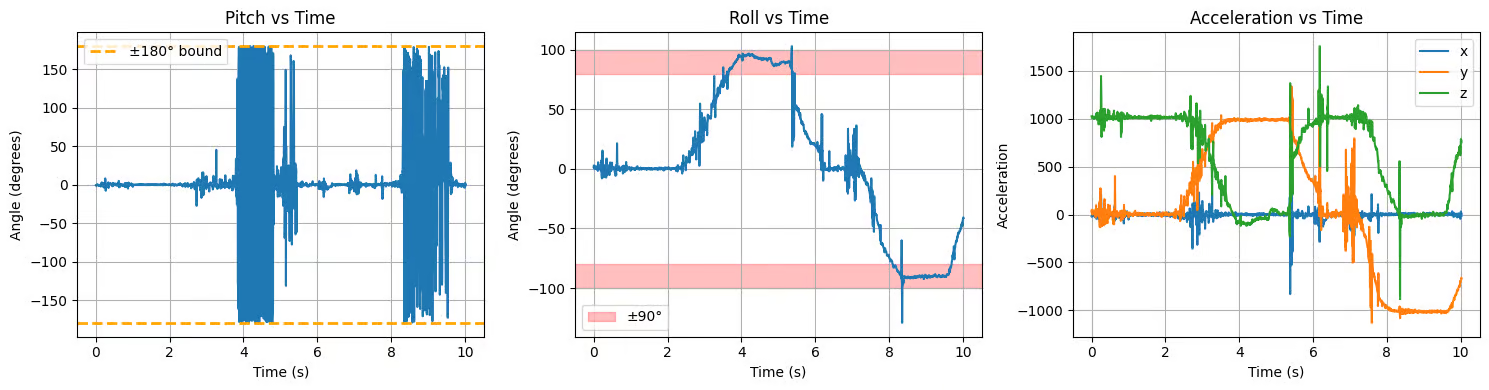
The output at {-90, 0, 90} degrees of roll behaves similarly:

Overall, the accelerometer provides accurate information. No two-point calibration is needed.

Frequency Spectrum Analysis

Using the scripy.fft library, I was able to graph the frequency spectrum of the pitch and roll data via Fourier transformation.

from scipy.fft import fft, fftfreq

dt = np.mean(np.diff(time))
freq = fftfreq(N, dt)[:N/frequency spectrum/2]

fft_raw_p = np.abs(fft(raw_pitch))
fft_raw_r = np.abs(fft(raw_roll))

fft_raw_p_norm = fft_raw_p[:N//2] / N
fft_raw_r_norm = fft_raw_r[:N//2] / N

plt.plot(freq, fft_raw_p_norm)
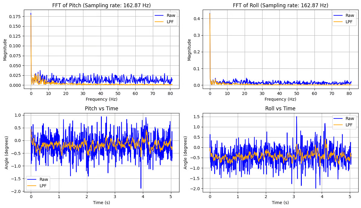
plt.plot(freq, fft_raw_r_norm)

Here is the frequency spectrum when I placed the sensor on the table.

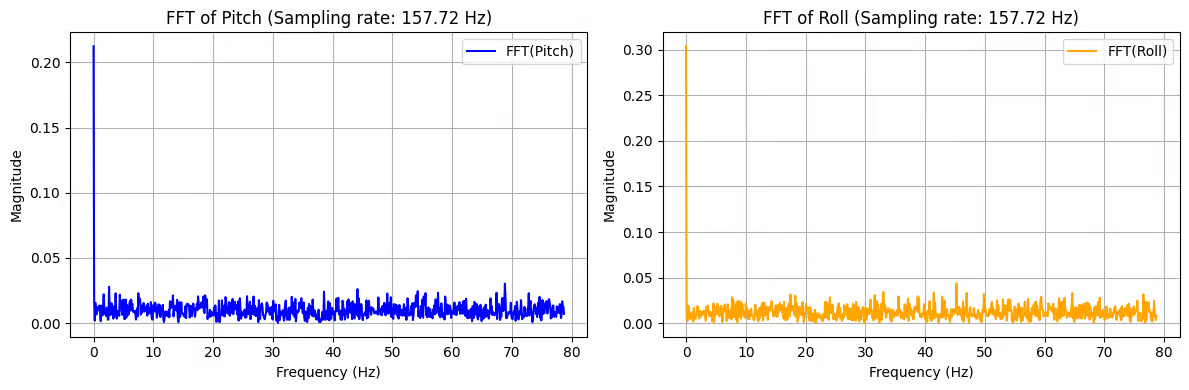
Both the pitch and roll spectra show a dominant spike at 0 Hz (DC component), which corresponds to the constant gravity-based orientation offset. Aside from this DC term, the remaining frequency content is relatively flat with a low noise floor across 0–80 Hz, and there are no strong resonant peaks.

This fairly smooth spectrum is caused by the internal filtering in the IMU data path,w which suppresses high-frequency noise before the data is transmitted

To further eliminate noise, I implemented additional first-order low-pass filter: $y[k]=y[k-1]+\alpha (x[k]-y[k-1])$.

I select $f_c= 5 Hz$ as the cutoff frequency based on the FFT plot. So, $\alpha = \frac{T}{T+RC}\approx 0,16$ with sampling rate $157.72 Hz$ for the low pass filter: $...$

I integrated this filter into the main loop so that each new accelerometer-derived pitch/roll estimate is filtered immediately after it is computed. I also added arrays to buffer samples.

if (myICM.dataReady()){
    // Other codes
    if (sample_count == 0){
        filt_acc_roll[sample_count] = raw_acc_roll[sample_count];
        filt_acc_pitch[sample_count] = raw_acc_pitch[sample_count];
    }
    else {
        filt_acc_roll[sample_count] = alpha * raw_acc_roll[sample_count] + (1 - alpha) * filt_acc_roll[sample_count-1];
        filt_acc_pitch[sample_count] = alpha * raw_acc_pitch[sample_count] + (1 - alpha) * filt_acc_pitch[sample_count-1];
    }
}

IIn the stationary case, the filter stabilizes and smooths the pitch in the time domain while limiting the frequency range. Most energy above 5 Hz is strongly attenuated.

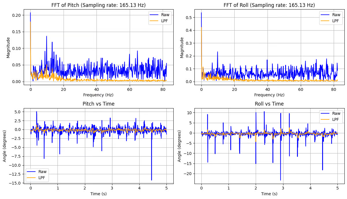
Then, I tested the filter effect by placing the IMU on a table and hitting it with my hand. This introduced sharp strikes in the time domain, which corresponded to broadband, high-frequency energy in the FFT spectrum. The LPF suppresses these high-frequency components and reduces the magnitude of sudden peaks.

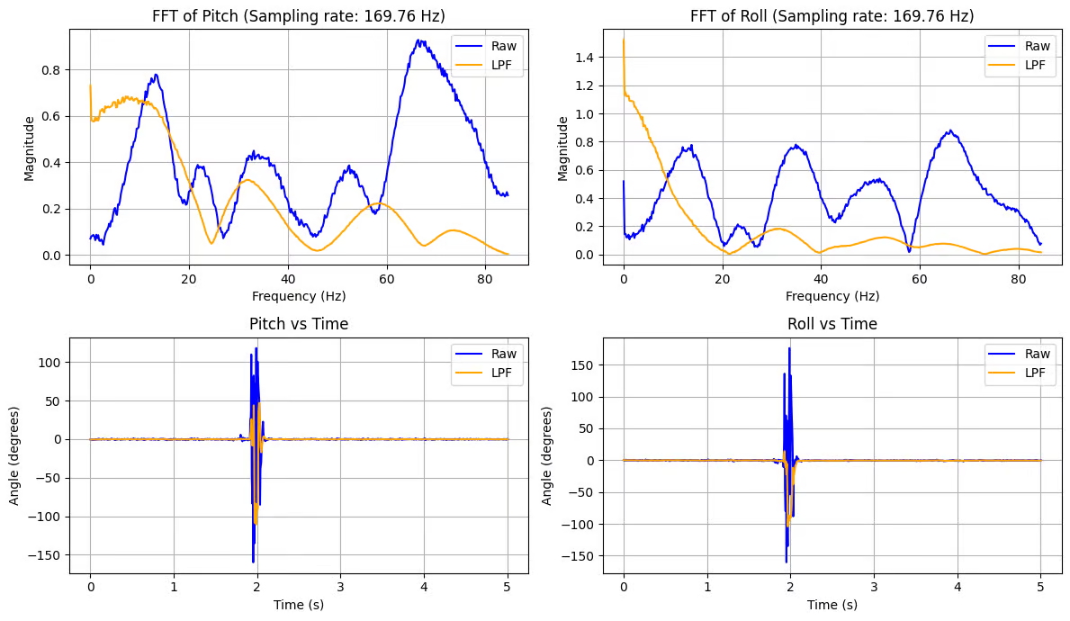
I tested the filter effect while the RC car was running nearby. The moving RC car generated periodic vibrations that produced multiple distinct peaks at mid-to-high frequencies in the FFT spectrum. The LPF reduces this oscillatory noise, resulting in a smooth, accurate output.

Gyroscope

I added the following code to the main loop to sample data from the gyroscope:

if (myICM.dataReady()){
    unsigned long current_sample_time = micros();
    float dt = (current_sample_time - last_sample_time)/1.e6;
    // Other codes

    if (sample_count == 0){
        // Other codes
        gyr_roll[sample_count] = myICM.gyrX()*dt;
        gyr_pitch[sample_count] = - myICM.gyrY()*dt;
        gyr_yaw[sample_count] = myICM.gyrZ()*dt;
    }
    else {
        // Other codes
        gyr_roll[sample_count] = myICM.gyrX()*dt + gyr_roll[sample_count-1];
        gyr_pitch[sample_count] = - myICM.gyrY()*dt - gyr_pitch[sample_count-1];
        gyr_yaw[sample_count] = myICM.gyrZ()*dt + gyr_yaw[sample_count-1];
    }
    sample_count++;
    last_sample_time = current_sample_time;
}

Here, the integration equation is used to compute the pitch, roll, and yaw angles: $\theta_g=\theta_g+\text{gyro_reading} * dt$

Besides, GET_GYRO_READINGS command is implemented to collect time-stamped gyroscope data and send to the host.

case GET_GYRO_READINGS:
    collecting = false;
    digitalWrite(LED_BUILTIN, LOW);

    for (int i = 0; i < sample_count; i++) {
        tx_estring_value.clear();
        tx_estring_value.append("T: ");
        tx_estring_value.append((int)time_buffer[i]);
        tx_estring_value.append("|r: ");
        tx_estring_value.append(gyr_roll[i]);
        tx_estring_value.append("|p: ");
        tx_estring_value.append(gyr_pitch[i]);
        tx_estring_value.append("|y: ");
        tx_estring_value.append(gyr_yaw[i]); 
        tx_characteristic_string.writeValue(tx_estring_value.c_str());
    }

Accuracy Discussion

First, I placed the sensor on the table to observe the static behavior.

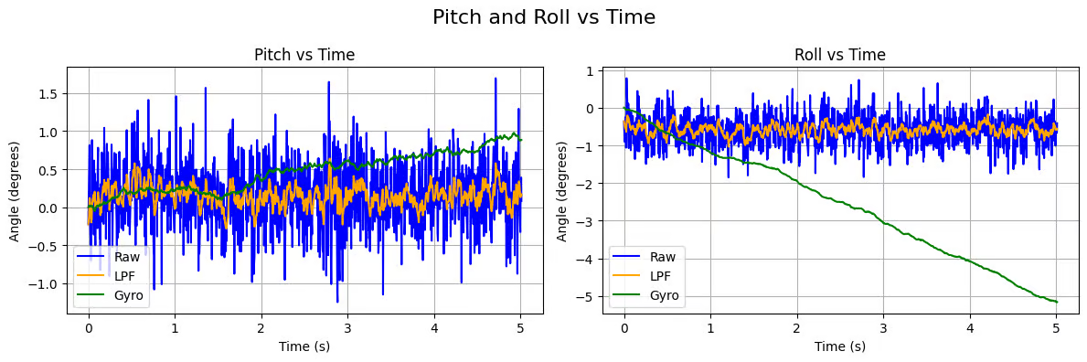
Compared with the accelerometer, the gyroscope output shows much less high‑frequency noise and almost no sudden spikes. However, because the angle is obtained by integrating angular velocity over time, even a small bias accumulates and produces a gradual drift. As a result, the gyro estimate slowly diverates from zero while the accelerometer (especially after low‑pass filtering) remains bounded around the true orientation.

Then I performed the same {−90°, 0°, 90°} rotations:

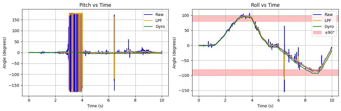
For rotation about the x‑axis, the roll estimated from the gyroscope follows the true motion closely with smooth transitions. The pitch channel remains stable, unlike the noisier accelerometer estimate. Similar for rotation about the y‑axis.

Frequency Discussion

Then, I increased SAMPLE_INTERVAL (in microseconds) from 3000 (333.33 Hz) to 30000 (33.33 Hz), and performed the {−90°, 0°, 90°} rotations.

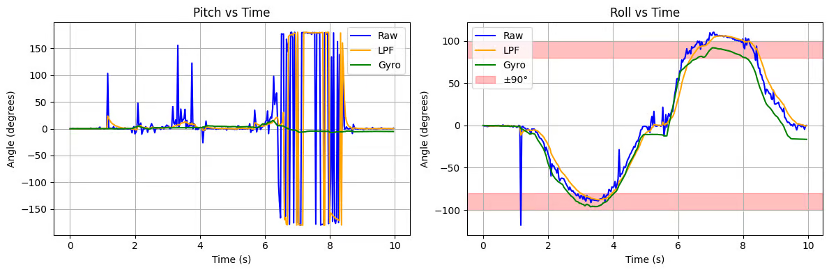
At lower sampling rate, noticeable drift and distortion appear, especially during fast motions. Then, the integrated gyroscope angles diverge more quickly over time.

Therefore, a higher sampling rate is necessary for reliable orientation tracking.

Complementary Filter

• During motion, the gyroscope response is smooth and tracks rapid changes accurately, while the accelerometer shows noticeable spikes caused by dynamic acceleration.
• After the motion stops, the accelerometer quickly settles to the correct absolute angle, whereas the gyroscope continues to drift slightly due to integration error.

Since the two sensors have complementary characteristics, we can use a complementary filter to combine them and achieve a more accurate result.

Here goes the equation: $\theta = (\theta+ \theta_g)(1-\alpha) + \theta_a\alpha$

I integrated it into the main loop and added a buffer array to sample the angles.

if (myICM.dataReady()){
    unsigned long current_sample_time = micros();
    float dt = (current_sample_time - last_sample_time)/1.e6;
    // Other codes

    if (sample_count == 0){
        // Other codes
        comp_roll[sample_count] = filt_acc_roll[sample_count]*alpha + gyr_roll[sample_count]*(1-alpha);
        comp_pitch[sample_count] = filt_acc_pitch[sample_count]*alpha + gyr_pitch[sample_count]*(1-alpha);
    }
    else {
        // Other codes
        comp_roll[sample_count] = filt_acc_roll[sample_count]*alpha + (1-alpha)*(comp_roll[sample_count-1] + myICM.gyrX()*dt);
        comp_pitch[sample_count] = filt_acc_pitch[sample_count]*alpha + (1-alpha)*(comp_pitch[sample_count-1] + myICM.gyrY()*dt);

    }
    sample_count++;
    last_sample_time = current_sample_time;
}

Besides, GET_COMP_READINGS command is implemented to collect time-stamped complementary-filtered data and send to the host.

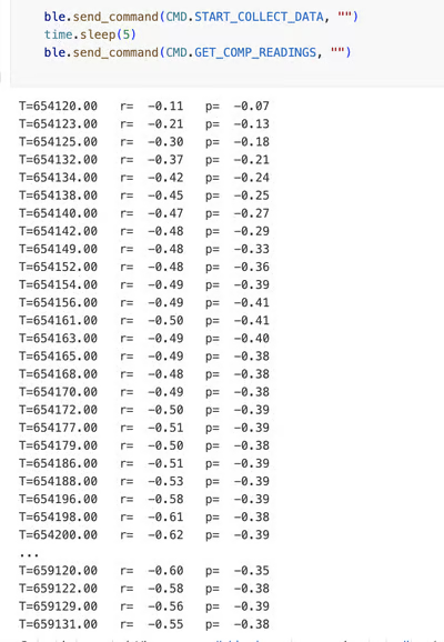
case GET_COMP_READINGS:
    collecting = false;
    digitalWrite(LED_BUILTIN, LOW);

    for (int i = 0; i < sample_count; i++) {
        tx_estring_value.clear();
        tx_estring_value.append("T: ");
        tx_estring_value.append((int)time_buffer[i]);
                tx_estring_value.append("|r: ");
                tx_estring_value.append(comp_roll[i]);
                tx_estring_value.append("|p: ");
                tx_estring_value.append(comp_pitch[i]);
        tx_characteristic_string.writeValue(tx_estring_value.c_str());
    }
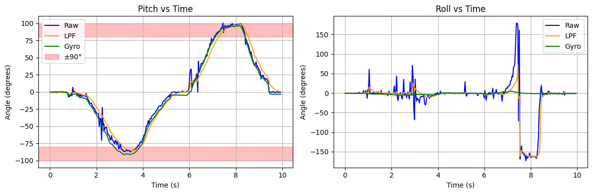
    break;

To check its working range and accuracy, I performed the same {−90°, 0°, 90°} rotations:

From the plots, the complementary filter output closely follows the true step changes while remaining significantly smoother than the raw accelerometer signal. During motion, the trajectory is continuous and free of large spikes, showing that the gyroscope term provides good short‑term tracking. When the board becomes stationary, the estimate quickly settles near the correct angle without long‑term drift, indicating that the accelerometer term corrects the accumulated gyro bias.

Compared with using either sensor alone, the fused result achieves both fast response and stable steady‑state accuracy, demonstrating improved robustness and reliability across the full working range.

Sample Data

Speed of Sample

I added a loop_count counter (incremented once per iteration) outside the IMU sampling block to measure how fast the main loop was actually running. Over the collection window, loop_count always matched sample_count. That is, every time the loop reached the sampling condition, myICM.dataReady() was already true and a new IMU measurement was available. The IMU output data rate is higher than the loop’s effective sampling rate, so the microcontroller loop becomes the limiting factor.

To speed up execution of main loop,

• I removed all the delays & Serial.print inserted for debugging。
• I checked the $myICM.dataReady()$ function to see if I should collect the sensor's data in the main loop.
• I minimized all unnecessary computations inside the loop and avoided dynamic memory allocation

As a result, the loop can run close to the hardware sampling limit of the IMU.

For a 5 s run, the board recorded 1337 samples, giving an effective sampling rate of $\approx 267 text{Hz}$ (≈ 270 Hz).

IMU data in Array

Instead of storing everything in one large struct array, I chose separate arrays for accelerometer- and gyroscope-derived signals.

• This allows for efficient access to operations such as filtering and offline analysis (FFT and plotting).
• Separate arrays provide the flexibility to enable and disable channels. When some components are no longer used, I can comment them out to save RAM without altering the overall data structure.
• This also makes the code more readable.

Datatype choice:

• Use unsigned long for time stamps. We need time in microseconds for computing dt and plotting.
• Use float for sensor value. IMU outputs and computed angles are real-valued. Float value ensure the enough precision for orientation estimation.
• Use int for counting (E.g. loop_count, sample_count). Using integers is compact and preserve full precision.

The RedBoard Artemis Nano has 384 KB RAM. Besides arrays, board also need memory for BLE stack, global objects, and call stacks/ local variables. So, $150-250KB$ could be a good range for array buffs.

My current buffer is about (SAMPLE_LEN = 3000):

• ime_buffer, temp_buffer
• `raw_acc_x/y/z'
• `raw_acc_roll/pitch'
• `gyr_roll/pitch/yaw'
• `filt_acc_roll/pitch'
• `comp_roll/pitch'

Total = 14 arrays × 3000 × 4 = 168,000 bytes ≈ 164 KB

5s of IMU Data

// Sample Buffer
const int SAMPLE_LEN = 3000;  

I set the maximum sample buffer size to 3,000. Since our sample rate is around 270 Hz, we can store over 10 seconds of IMU data.

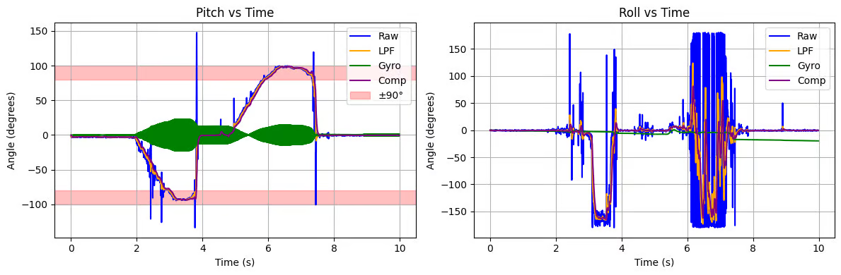
Record a stunt

After playing around with the car, I found that I could make it flip over by quickly switching between forward and backward. This feature allows the car to perform an emergency stop or turn back. The board may recognize this kind of motion if there are significant changes in the IMUs.

Video Here

Collabration

I referenced Lucca’s and Stephan's site for code debugging and graph formatting. I used ChatGPT for graph plotting and website formatting/development.