The objective of this lab is to implement a Kalman Filter to improve state estimation for the robot’s motion, enabling faster and more accurate control.
Task 1. Estimate Drag and Momentum
To estimate the drag and momentum terms required for constructing the state-space model (A and B matrices), I performed a step response experiment by driving the robot toward a wall at a constant high motor input (100% PWM). During this run, I logged ToF distance measurements and computed velocity using a finite difference approximation: $v = \frac{\Delta \text{distance}}{\Delta t}$. The experiment was repeated three times to improve robustness and reduce noise effects.
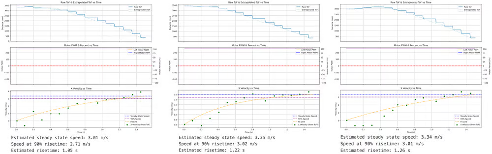
From the recorded data, I extracted key dynamic characteristics:
- Average steady-state speed: $v_{ss} = 3.24 m/s$
- Average 90% rise time: $t_{0.9} = 1.17 s$
- Speed at 90% rise time :$v_{0.9} = 2.91 m/s$
Assuming a first-order system model, the drag coefficient $d$ can be approximated from the steady-state relationship between input and velocity: $d = \frac{u}{v_{ss}},$ where $u \in [0,1]$ represents the normalized motor input. Using $u = 1$, we obtain: $d ≈ \frac{1}{3240 mm/s} ≈ 3.09 × 10^{-4}$.
The momentum coefficient $m$ is then estimated using the rise time relationship for a first-order system: $m = \frac{-d \cdot t_{0.9}}{\ln(1 - 0.9)} ≈ 1.58 × 10^{-4}$.
Task 2. Initialize KF in Python
Using the estimated drag and momentum coefficients, the continuous-time state-space model is defined as:
$A = \begin{bmatrix} 0 & 1 \ 0 & -\frac{d}{m} \end{bmatrix}$,
$B = \begin{bmatrix} 0 \ \frac{1}{m} \end{bmatrix}$.
Substituting the estimated values gives: $A \approx \begin{bmatrix} 0 & 1 \ 0 & -1.96 \end{bmatrix}, B\approx \begin{bmatrix} 0 \ 6348.45494 \end{bmatrix}$.
To implement the Kalman Filter, the system is discretized using a sampling time dt. Based on a 5-second run with approximately 474 control loop iterations, the sampling time is:
$dt ≈ 0.01 s$.
The discrete-time matrices are computed as:
Ad = np.eye(2) + dt * A
Bd = dt * B
The measurement matrix is defined as:
C = np.array([[-1, 0]])This reflects that the ToF sensor measures distance (with sign convention opposite to the state definition).
The initial state is set as:
x = np.array([[-tof_values[0]], [0]])which assumes the robot starts at the initial measured distance with zero velocity.
Next, the process noise covariance ($\Sigma_u$) and measurement noise covariance ($\Sigma_z$) are defined.
For the process noise, I assumed approximately 10 mm uncertainty over 1 second, leading to $\sigma_1 = \sigma_2 = \sqrt{\frac{100}{dt}}\approx 95$. Then:
sigma_u = np.array([[95**2, 0],
                    [0, 95**2]])
For the measurement noise, I recorded ToF data at a fixed distance (~3 m) and computed a standard deviation of approximately 15.96 mm, giving:
sigma_z = np.array([[16**2]])Also, the initial state covariance matrix is set as:
Sigma = np.array([[100**2, 0],[0, 100**2]])which reflects a relatively high initial uncertainty in both position and velocity estimates, allowing the filter to rely more on incoming measurements during the initial phase.
Finally, the Kalman Filter is implemented following the standard predict-update formulation, where the update parameter controls whether a measurement update is performed or only the prediction step is executed:
def kf(mu, sigma, u, y, update=True):
    mu_p = Ad.dot(mu) + Bd.dot(u)
    sigma_p = Ad.dot(sigma.dot(Ad.transpose())) + sigma_u

    if not update:
        return mu_p, sigma_p

    sigma_m = C.dot(sigma_p.dot(C.transpose())) + sigma_z
    kkf_gain = sigma_p.dot(C.transpose()).dot(np.linalg.inv(sigma_m))

    y_m = y - C.dot(mu_p)
    mu = mu_p + kkf_gain.dot(y_m)
    sigma = (np.eye(2) - kkf_gain.dot(C)).dot(sigma_p)

    return mu, sigma
Task 3: Implement and test Kalman Filter in Python
To verify the parameters, I used the experience data from Lab 5 to test Kalman Filter.
I implemented the loop to apply the Kalman filter to all the data in Lab 5.
kf_positions = []
kf_velocities = []
last_tof_val = None
for i in range(len(t_s)):
current_u = np.array([[u_raw[i]]])
current_y = np.array([[tof_2_values[i]]])
if tof_update[i]:
mu, sigma = kf(mu, sigma, current_u, current_y, update=True)
else:
mu, sigma = kf(mu, sigma, current_u, current_y, update=False)
kf_positions.append(mu[0, 0])
kf_velocities.append(mu[1, 0])
kf_positions = np.array(kf_positions)
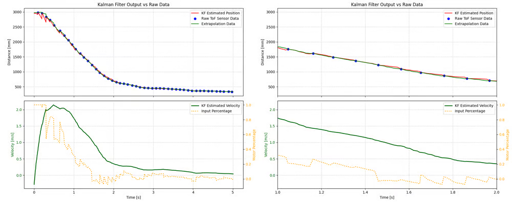
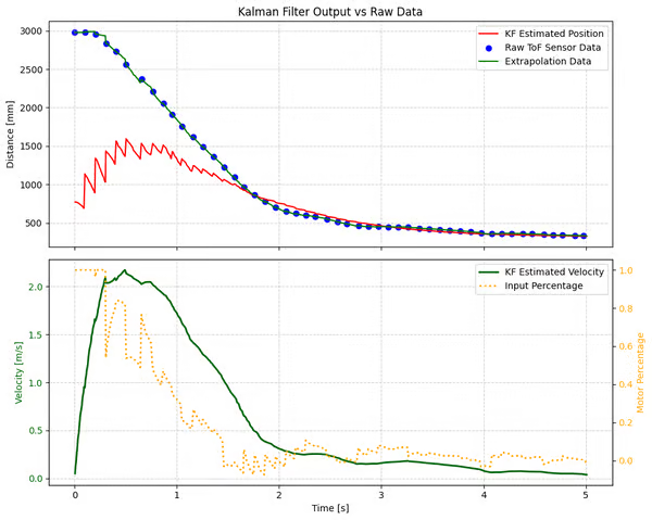
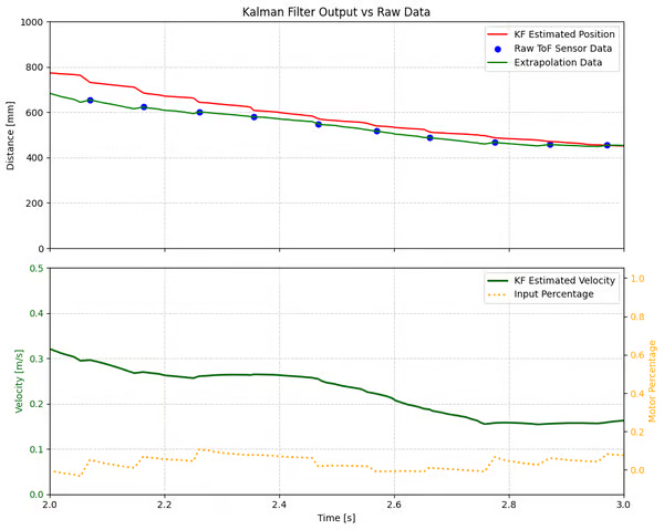
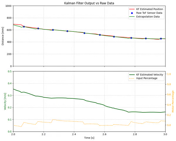
kf_velocities = np.array(kf_velocities)Using the pre-calculated parameters, the Kalman Filter produces stable and physically consistent estimates of both position and velocity. The comparison between raw ToF data, extrapolated data, and Kalman Filter output is shown in the figure.
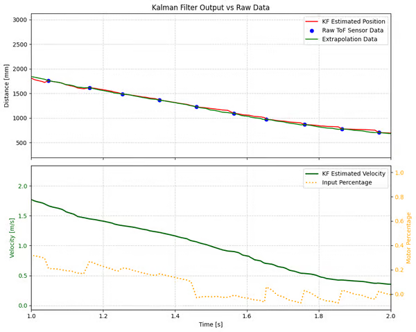
From the position plot (and zoomed-in one on the right), the KF estimated position closely follows the discrete ToF measurements while providing a continuous trajectory between updates. Compared to simple extrapolation, the Kalman Filter is less sensitive to noise and avoids sharp jumps when new sensor data arrives.
From the velocity plot (and zoomed-in one on the right), the KF estimated velocity exhibits a smooth, continuous and realistic trend.
Therefore, the Kalman Filter significantly improves state estimation compared to both raw sensor data and linear extrapolation, especially under low sampling rate conditions of the ToF sensor.
Parameters Discussion
-
Drag $d$ and Momentum $m$ Coefficients: tell the filter how fast and how far the robot should be traveling at a given PWM level.
-
Process Noise Covariance Matrix $\Sigma_u$: confidence for the mathematical state-space model.
-
If the model is overconfidence ($\Sigma_u$ too small), it will disregard the sensor's actual readings and lead to large bias.
-
If the model is underconfidence ($\Sigma_u$ too large),it rduced to a simple sensor-based prediction model (Extrapolation).
-
-
Measurement Noise Covariance $\Sigma_z$: uncertainty for the ToF sensor.
-
If $\Sigma_z$ is set too large, the filter will interpret the sensor data as being full of noise and will ignore new data. This results in an extremely smooth red line, but with significant lag.
-
If $\Sigma_z$ is set too small, the filter treats every minor fluctuation in the ToF data as valid, thereby negating the purpose of filtering.
-
Task 4: Implement the Kalman Filter on the Robot
The global variables define the system dynamics ($A, B$), state estimate ($\mu$), and uncertainty ($\Sigma$), as well as the process and measurement noise covariances. These parameters are pre-computed from the system identification step and remain constant during execution. The matrices are implemented using the BasicLinearAlgebra library to enable efficient matrix operations on the microcontroller.
#include <BasicLinearAlgebra.h>
using namespace BLA;
float sys_d = 0.000309f;
float sys_m = 10.579281f;

Matrix<2, 2> A = {0.0f, 1.0f, 0.0f, -sys_d / sys_m};
Matrix<2, 1> B = {0.0f, 1.0f / sys_m};

Matrix<2, 1> mu = {0.0f, 0.0f};
Matrix<2, 2> Sigma = {10000.0f, 0.0f, 0.0f, 10000.0f};

Matrix<1, 2> C = {1.0f, 0.0f};
// Process Noise
Matrix<2, 2> Sigma_u = {97.0f * 97.0f, 0.0f, 0.0f, 97.0f * 97.0f};
// Measurement Noise
Matrix<1, 1> Sigma_z = {15.0f * 15.0f};

Matrix<2, 2> I2 = {1.0f, 0.0f, 0.0f, 1.0f};
The function getEstimateValue(dt) implements the predict-update cycle of the Kalman Filter in real time.
float getEstimateValue(float dt){
    if (kalman_filter){
        Matrix<2, 2> Ad = I2 + A * dt;
        Matrix<2, 1> Bd = B * dt;
        float u_t = output_value / 100.0f;
        Matrix<1, 1> u_vec = {u_t};
        Matrix<2, 1> mu_p = Ad * mu + Bd * u_vec;
        Matrix<2, 2> Sigma_p = Ad * Sigma * (~Ad) + Sigma_u;
        if (!sensor_updated)
        {
            mu = mu_p;
            Sigma = Sigma_p;
            return mu_p(0, 0);
        }
        Matrix<1, 1> y = {tof2_dist};
        Matrix<1, 1> y_m = y - C * mu_p;
        Matrix<1, 1> S = C * Sigma_p * (~C) + Sigma_z;
        Matrix<1, 1> S_inv;
        S_inv(0, 0) = 1.0f / S(0, 0);
        Matrix<2, 1> K = Sigma_p * (~C) * S_inv;
        mu = mu_p + K * y_m;
        Sigma = (I2 - K * C) * Sigma_p;
        return mu(0, 0);
    }
    // .......
}
The Kalman Filter is then integrated into the PID controller by replacing the raw ToF measurement with the estimated state.
void runController(){
float new_estimate = getSensorValue(dt);
float new_error = new_sensor - setpoint;
derivative_value = mu(1, 0);
// Anti-Windup
raw_integral_value = integral_value + new_error * dt;
float new_integral = constrain(raw_integral_value, -integral_limit, integral_limit);
float unsat_output = kp * new_error + ki * new_integral + kd * derivative_value;
bool saturated_high = unsat_output > output_limit;
bool saturated_low = unsat_output < -output_limit;
if ((!saturated_high && !saturated_low) || (saturated_high && new_error < 0) || (saturated_low && new_error > 0))
{
integral_value = new_integral;
}
output_value = kp * new_error + ki * integral_value + kd * derivative_value;
error_value = new_error;
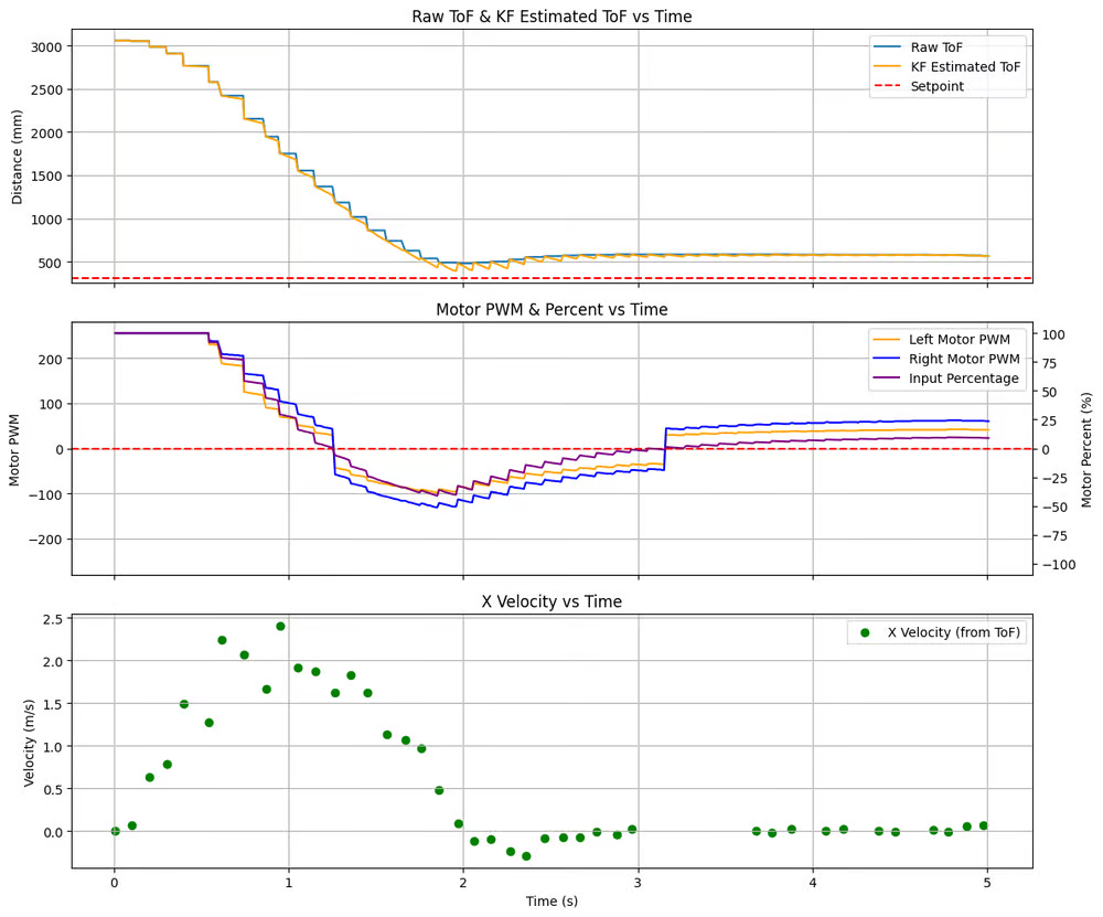
}After implementation, the Kalman Filter-based controller successfully operated on the robot and demonstrated clear improvements over the previous extrapolation-based approach.
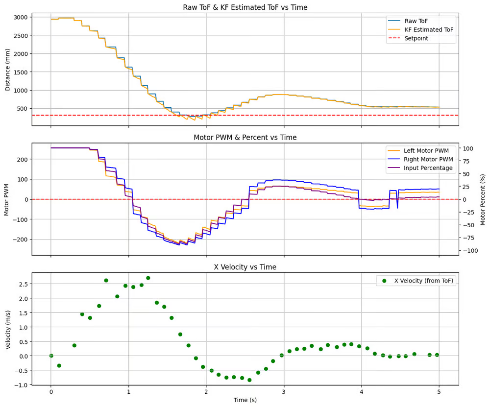
From the KF-based run, the estimated ToF (orange) closely follows the raw ToF measurements while remaining smooth and continuous. Although a small overshoot is observed after reaching the target distance, the system quickly stabilizes.
The motor PWM plot shows that the control signal is significantly smoother compared to the extrapolation-based method. The PWM values in KF-based run change gradually and continuously, indicating that the controller receives a more reliable state estimate (both position and velocity). This reduces aggressive oscillations and prevents abrupt motor commands.
Here is data from lab5 where using extrapolation we can compare with:
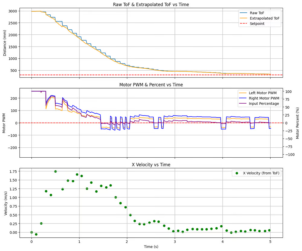
We can see that the KF-based run is much faster while keeping the ToF trajectory as smooth as the extrapolation-based run.
The extrapolation-based run also shows noticeable oscillations in both PWM and estimated distance. The extrapolated position introduces noise and discontinuities, especially when ToF updates are sparse, which leads to rapid fluctuations in control output.
Overall, integrating the Kalman Filter results in smoother trajectories, more stable control signals, and improved responsiveness, especially under low sensor update rates. This demonstrates the advantage of combining model-based prediction with noisy sensor measurements in real-time robotic control.
Task 5: Speed Up
To reduce the overshoot and oscillation observed in Task 4 while maintaining fast response, I re-tuned the PID controller after integrating the Kalman Filter.
The previous gains ($K_p = 0.05, K_i = 0, K_d = 0.05$) became too aggressive, leading to overshoot and oscillatory behavior near the setpoint.
To address this, I reduced $K_p$ slightly to decrease the overall control aggressiveness. At the same time, I reduced $K_d$ because the derivative term is now computed from the Kalman Filter’s smooth velocity estimate, making a large derivative gain unnecessary and potentially amplifying small fluctuations.
The final tuned parameters are: $K_p = 0.043,\quad K_i = 0,\quad K_d = 0.04$.
With these gains, the system achieves a good balance between responsiveness and stability, improving the damping behavior.
Later, $K_i$ may be introduced to solve the steady error problem.