The objective of this lab is to integrate sensing, control, and actuation into a unified system capable of executing a fast “flip” stunt, where the robot drives forward at high speed, performs a flip near the wall, and returns past the starting line.
PID Controller
For my previous lab code, there's a single shared PID state that can only do distance OR orientation at a time. For the flip stunt, however, forward motion and heading stabilization needed to operate simultaneously, so I refactored the controller into a PIDController struct that encapsulates the PID gains, internal states, sensor estimation logic, and a reusable compute() method.
The PIDController struct also supports three sensing modes—direct measurement, extrapolation, and Kalman filtering for flexibility.
struct PIDController
{
    // --- PID Gains, States, Tunings ---
    // ---------------------------------

    // --- Extrapolation States ---
    // ---------------------------------

    // --- Kalman Filter States ---
    // ---------------------------------

    // --- Sensor Estimation Mode ---
    enum SensorMode
    {
        DIRECT,
        EXTRAPOLATION,
        KALMAN
    };


    // --- Helper Functions for Kalman Filter  ---
    // ---------------------------------

    // --- Helper Functions for Extrapolation  ---
    // ---------------------------------

    // --- Unified Sensor Estimate ---
    float getEstimate(float raw_measurement, bool has_new_measurement, float dt);
        // DIRECT:        returns raw_measurement
        // EXTRAPOLATION: returns getExtrapolated(micros())
        // KALMAN:        calls kfPredict(dt), kfUpdate if new, returns kfPosition()


    // --- PID Core ---
    void reset();
        // Zeros all PID state + extrapolation state, count = 0
        // (Does NOT reset gains, setpoint, tuning params, or KF model)

    float compute(float new_sensor, float dt, bool wrap_angle = false, bool use_kf_derivative = false);
        // 1. Error:
        //      wrap_angle=false → error = new_sensor - setpoint
        //      wrap_angle=true  → error = wrapAngle180(new_sensor - setpoint)
        //
        // 2. Derivative:
        //      use_kf_derivative=true  → uses kfVelocity() directly
        //      use_kf_derivative=false → d/dt on measurement + LPF
        //
        // 3. Integral:  with conditional anti-windup
        //      raw  = integral + error × dt
        //      clamped to [-integral_limit, integral_limit]
        //      only integrates when output not saturated in error direction
        //
        // 4. Output:
        //      kp·error + ki·integral + kd·derivative
        //      clamped to [-output_limit, output_limit]
        //
        // Returns: output_value
};
This design allows multiple independent controllers to run in parallel. Distance Controller and Orientation Controller can be initialized as following:
// Distance PID — controls forward/backward via ToF
PIDController dist_pid;
// Orientation PID — controls turning via IMU yaw
PIDController orient_pid;
I could separately tune forward and angular control like this:
float estimate = dist_pid.getEstimate(tof2_dist, tof_updated, dt);
bool use_kf_d = (dist_pid.sensor_mode == PIDController::KALMAN);
dist_pid.compute(estimate, dt, false, use_kf_d);
applyLinearOutput(dist_pid.output_value);
float new_sensor = getOrientationSensorValue();
orient_pid.compute(new_sensor, dt, true);
applyAngularOutput(-orient_pid.output_value);New commands are added for tuning and changing setpoint via BLE:
UPDATE_DIST_PID,UPDATE_ORIENT_PIDSET_DIST_SETPOINT,SET_ORIENT_SETPOINT
Motor Mixing
To test the controller in a high-speed scenario, I implemented a MODE_RUSH behavior that drives the robot forward aggressively while using the orientation PID loop to maintain a straight trajectory.
In this mode, the forward command is held at a fixed high value, while the angular correction from orient_pid is mixed into the left and right motor commands with opposite signs.
void runController(){
    // ---------------------------------
    case MODE_RUSH:
    {
        float estimate = dist_pid.getEstimate(tof2_dist, tof_updated, dt);
        dist_pid.sensor_value = estimate;
        dist_pid.output_value = 100.0f;
        float orient_sensor = getOrientationSensorValue();
        float angular = orient_pid.compute(orient_sensor, dt, true);

        float left_raw = 100.0f - angular;
        float right_raw = 100.0f + angular;
        float max_raw = max(left_raw, right_raw);
        if (max_raw > 100.0f)
        {
            float overshoot = max_raw - 100.0f;
            left_raw -= overshoot;
            right_raw -= overshoot;
        }
        left_motor_pct = constrain(left_raw * MOTOR_SCALE, -100.0f, 100.0f);
        right_motor_pct = constrain(right_raw * MOTOR_SCALE, -100.0f, 100.0f);
        setMotors(left_motor_pct, right_motor_pct);
        break;
    }
    // ---------------------------------
}
The robot was tested over a 4 m trajectory at maximum speed. Unlike previous labs (5& 7) where distance PID combined with open-loop orientation control led to significant drift at this range, the current approach achieves substantially improved stability.
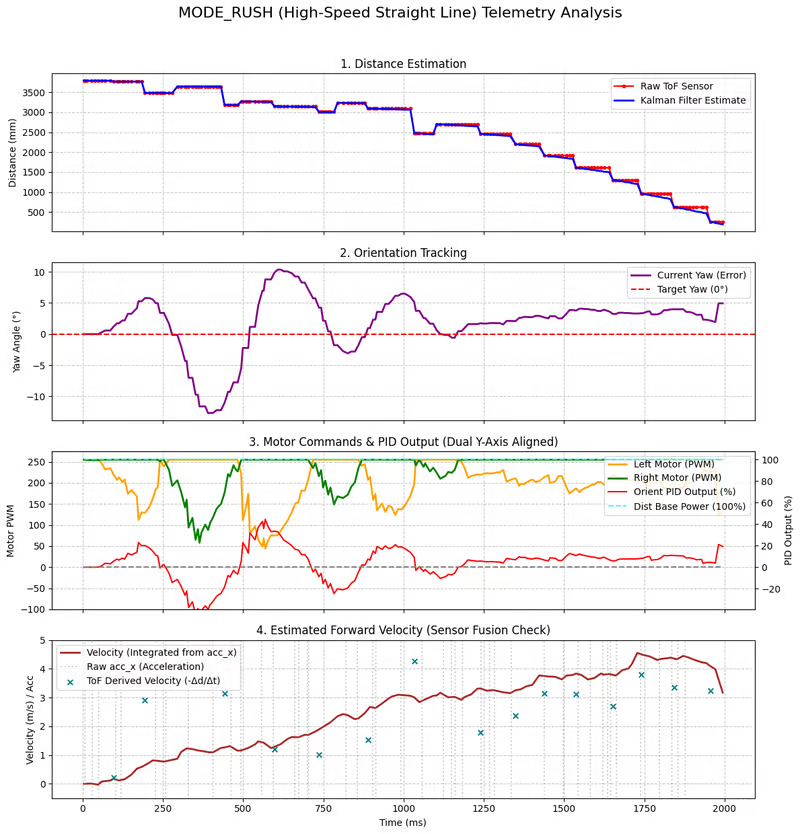
From the orientation tracking plot, the yaw error remains tightly bounded within approximately ±2°. At the same time, the velocity estimation shows that the robot reaches a peak steady speed of approximately 3.2 m/s (similary to lab7), demonstrating that high-speed performance is maintained without sacrificing stability.
Flips
For the flip task, I abandoned closed-loop distance control near the wall and instead applied a fixed, very high PWM command in open loop so that the robot could sprint forward at maximum speed. Heading control is active to keep the robot moving approximately straight toward the target region and backward after flipping.
Kalman Filter Update
To improve distance estimation at high speed, I kept the Kalman filter running in an asynchronous update mode. When a new ToF measurement was available, the controller executed both the prediction and update steps. When no new sensor reading was available, it executed only the prediction step, propagating the state estimate forward using the dynamics model and motor input.
Because the control loop frequency changed significantly in this mode, I updated the discrete-time model accordingly. The control loop now runs at about 500 iterations in 5 seconds, so I set $dt = 0.01s$ and recomputed the discrete system matrices using
Ad = np.eye(2) + dt * A
Bd = dt * B
The average steady-state speed, average 90% rise time, and speed at the 90% rise time remained consistent with the values obtained in Lab 7.
Code Implementation
The flip behavior was implemented as a finite-state machine with four stages:
FLIP_READYFLIP_STARTEDFLIP_RECOVERFLIP_RETURN
In FLIP_READY, the robot drives forward at maximum power while the orientation PID provides small steering corrections to maintain a straight trajectory. During this phase, the Kalman-filtered distance estimate is monitored continuously. Once the estimated distance falls below the chosen trigger threshold, the robot transitions into the flip phase.
if (flip_state == FLIP_READY)
{
    dist_pid.output_value = 100.0f;
    float angular = orient_pid.compute(orient_sensor, dt, true);

    left_motor_pct = constrain((100.0f - angular) * MOTOR_SCALE, -100.0f, 100.0f);
    right_motor_pct = constrain((100.0f + angular) * MOTOR_SCALE, -100.0f, 100.0f);
    setMotors(left_motor_pct, right_motor_pct);

    if (dist_estimate <= dist_pid.setpoint)
    {
        flip_state = FLIP_STARTED;
        flip_time = current_control_time;
    }
}
In FLIP_STARTED, both motors are immediately driven at full reverse power. So sharp torque change is created to initiate the flip. The IMU roll angle is used to detect when the robot has rotated enough to confirm that the flip has begun.
else if (flip_state == FLIP_STARTED)
{
    dist_pid.output_value = -100.0f;
    left_motor_pct = -100.0f * MOTOR_SCALE;
    right_motor_pct = -100.0f * MOTOR_SCALE;
    setMotors(left_motor_pct, right_motor_pct);
    if (abs(dmp_roll) > 50.0f)
    {
        flip_state = FLIP_RECOVER;
        flip_time = current_control_time;
    }
}
In FLIP_RECOVER, the motors are temporarily stopped so the robot can complete the rotation and settle after impact. The roll angle is again monitored, and once it approaches an fully rotated posture, the controller transitions to the return phase. At this point, the yaw reference is reset and the Kalman filter is reinitialized using the new measured distance.
else if (flip_state == FLIP_RECOVER)
{

    dist_pid.output_value = 0.0f;
    left_motor_pct = 0.0f;
    right_motor_pct = 0.0f;
    setMotors(left_motor_pct, right_motor_pct);

    if (abs(dmp_roll) > 175.0f)
    {
        flip_state = FLIP_RETURN;
        yaw_offset = dmp_yaw;
        orient_pid.reset();
        float new_start_dist = (tof2_dist > 10.0f) ? tof2_dist : 3000.0f;
        dist_pid.resetKalman(new_start_dist);
    }
}
In FLIP_RETURN, the robot drives back at high speed in the opposite direction. Orientation PID is re-enabled so that the robot can maintain a stable heading while retreating away from the wall and crossing back over the starting line.
else if (flip_state == FLIP_RETURN)
{
    dist_pid.output_value = -100.0f;
    float angular = -orient_pid.compute(orient_sensor, dt, true);
    left_motor_pct = constrain(-(100.0f - angular) * MOTOR_SCALE, -100.0f, 100.0f);
    right_motor_pct = constrain(-(100.0f + angular) * MOTOR_SCALE, -100.0f, 100.0f);
    setMotors(left_motor_pct, right_motor_pct);
}
Lead Time Tuning
Because of otor response delay and the robot’s high forward speed, the robot cannot stop or reverse exactly at the nominal 1 ft (304 mm) target location in real time. I tuned the trigger setpoint to 1000 mm, such that the robot has enough time to process and flip at the target location.
Trial 1
Trial 2
Trial 3
Flip Results & Discussion
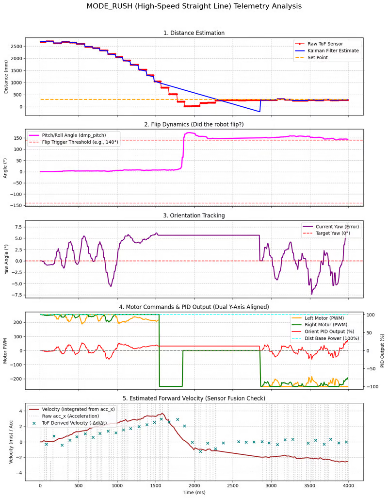
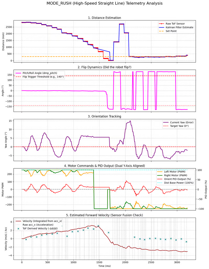
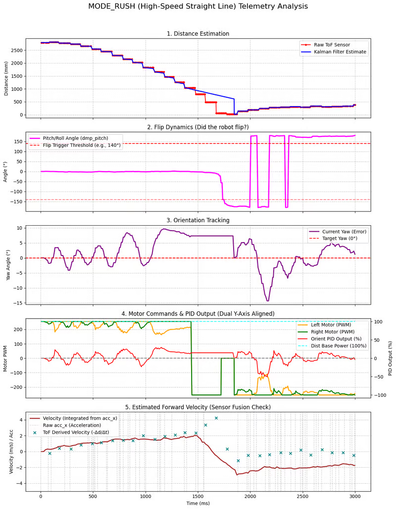
Across three successful trials, the robot consistently achieved a maximum forward speed of approximately $3 m/s$ during the approach phase and about $2 m/s$ during the return phase over a $~3 m$ travel distance. The backward velocity was estimated from the integrated acceleration in the x-direction, since reliable ToF measurements were not available after the flip. The total time for a complete forward–flip–return cycle was approximately $3.5$ seconds.
From the plots, the flip event is clearly captured by a sharp transition in the roll/pitch angle, exceeding the flip detection threshold (~140°), confirming that a full rotation occurred. After recovery, the robot resumes controlled backward motion with orientation stabilization re-enabled. Orientation tracking remains reasonably bounded despite the aggressive maneuver, indicating that the angular PID controller continues to function effectively.
A key limitation observed in this lab is the use of a single front-facing ToF sensor. Although I tried to align the sensor parallel to the ground, after the flip the sensor often points toward the floor instead of the wall, resulting in invalid or misleading distance readings. This is evident in the distance estimation plots, where the ToF signal becomes unreliable immediately after the flip. As a result, post-flip control relies less on distance feedback and more on open-loop behavior and IMU-based stabilization.
For future improvements, I reconsider the sensor placement strategy . Instead of mounting a second ToF sensor on the side, a more effective approach would be to mount an additional sensor at the rear of the robot with a slight downward angle. This configuration would allow the robot to maintain valid distance measurements relative to the wall even after flipping, enabling more robust closed-loop control during the return phase.
Blooper
Here’s a blooper video where I tried the flip on a smooth floor. The robot ended up drifting around pretty chaotically after the flip, since there wasn’t enough friction to keep it stable. But somehow, it still managed to make its way back and cross the starting line in the end $:)$