Posted on 2026-04-15

This lab focuses on constructing a geometric map of a static indoor environment using the robot equipped with ToF sensors and IMU. The robot is placed at multiple known locations and performs in-place rotations to collect distance measurements. Spatial representation is generated by transforming these local sensor readings into a global reference frame.

Orientation Control

I chose orientation-based PID control for mapping, as it provides more consistent angular spacing between measurements compared to open-loop control. To implement this, I designed a finite state machine that ensures accurate rotation, stabilization, and reliable sensor acquisition at each step.

The mapping process consists of the following states:

MAP_START: Initialize the mapping procedure by recording the starting orientation, resetting the PID controller, and setting the first step.

case MAP_START:
    map_start_angle = orient_sensor;
    map_step = 1;
    orient_pid.reset();
    map_state = MAP_TURN;
    break;

MAP_TURN: Rotate the robot toward the next target angle using the orientation PID controller.

case MAP_TURN:
{
    float target_angle = map_start_angle + (map_step * map_increment);
    orient_pid.setpoint = target_angle;

    float angular = orient_pid.compute(orient_sensor, dt, false);
    applyAngularOutput(-angular);

    if (abs(orient_pid.error_value) < 3.0f)
    {
        map_state = MAP_STABILIZE;
        map_stabilize_time = current_control_time;
    }
    break;
}

MAP_STABILIZE: Hold the robot at the target angle for a short duration to reduce motion-induced ToF noise.

case MAP_STABILIZE:
{
    float target_angle = map_start_angle + (map_step * map_increment);
    orient_pid.setpoint = target_angle;
    float angular = orient_pid.compute(orient_sensor, dt, false);
    applyAngularOutput(-angular);

    if (current_control_time - map_stabilize_time > 500000)
    {
        applyAngularOutput(0.0f);
        wait_tof1_ready = false;
        wait_tof2_ready = false;
        map_state = MAP_MEASURE;
    }
    break;
}

MAP_MEASURE: Collect synchronized readings from both ToF sensors once the robot is stationary. After measurement, go back to MAP_TURN to continue rotation or jump to MAP_DONE to complete mapping

case MAP_MEASURE:
{
    applyAngularOutput(0.0f);
    if (tof1_updated)
        wait_tof1_ready = true;
    if (tof2_updated)
        wait_tof2_ready = true;

    if (wait_tof1_ready && wait_tof2_ready)
    {
        valid_map_tof1 = tof1_dist;
        valid_map_tof2 = tof2_dist;
        map_step++;

        wait_tof1_ready = false;
        wait_tof2_ready = false;

        if (map_step * map_increment >= map_total_degrees)
            map_state = MAP_DONE;

        else
            map_state = MAP_TURN;
    }
    break;
}

MAP_DONE: Perform a final correction to the full rotation angle and terminate the mapping process.

case MAP_DONE:
{
    orient_pid.setpoint = map_start_angle + map_total_degrees;
    float angular = orient_pid.compute(orient_sensor, dt, false);
    applyAngularOutput(-angular);
    if (abs(orient_pid.error_value) < 5.0f || (millis() - start_sample_time >= SAMPLE_DURATION))
    {
        if (tof1_updated && tof2_updated)
        {
            applyAngularOutput(0.0f);
            valid_map_tof1 = tof1_dist;
            valid_map_tof2 = tof2_dist;
            active = false;
        }
    }
    break;
}

The PID controller was tuned in Lab 6 with parameters: $K_p = 2.5, \quad K_i = 1.2, \quad K_d = 0.25$

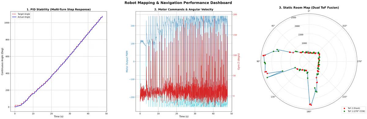
The following test confirms that the robot performs approximately on-axis $360-$degree rotations with $20-$degree increments, which is critical for accurate mapping.

Video Here

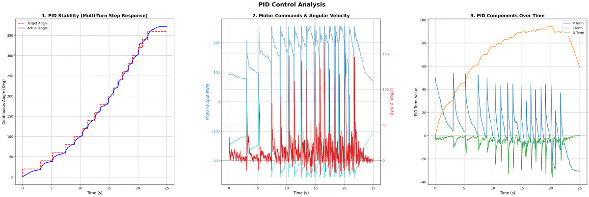
The step response (left) shows that the robot closely follows the target angle at each increment, with small steady-state error and minimal overshoot.

The PID term plot (right) reveals that

The P term dominates during transitions, providing fast response.
The I term gradually accumulates to eliminate steady-state error.
The D term helps damp oscillations, though it remains relatively small due to filtering and noise sensitivity

Overall, the controller is stable and responsive, with no sustained oscillations or divergence across multiple turns.

Error ad Accuracy Analysis

The robot maintains good rotational accuracy that the maximum positional drift from the origin is within 5 cm.

Based on prior calibration (Lab 3), the ToF sensor has: $\approx 30\text{ mm}$ error for distances $\leq 2\text{ m}$ and up to $\approx 200 \text{ mm}$ error for distances between $2–3.5 \text{m}$.

Assuming the robot performs an on-axis rotation in the center of a $4 \text{m} × 4 \text{m}$ room:

The average radial measurement error is $\approx 0.05 - 0.1 m$ (at short range)
The worst-case radial measurement error is $\approx 0.20 - 0.25 m$ (at long range)

Though the actual angle increments are roughly $20-$degrees for most steps, slight overshoot still occurs during some transition, so it is better use the orientation from gyoscope for graphing.

Transformation Matrices

Before collecting distance measurements in the lab space, I first calibrated the coordinate system so that the polar plot orientation aligns with the robot’s frame. In this setup, the robot rotates counterclockwise (CCW), and the yaw angle from the IMU is used directly as the heading of the robot.

To convert ToF measurements into global coordinates, I used a 2D rigid body transformation, expressed in homogeneous coordinates:

$$T(\theta, x_r, y_r) = \begin{bmatrix} \cos\theta & -\sin\theta & x_r \ \sin\theta & \cos\theta & y_r \ 0 & 0 & 1 \end{bmatrix}$$

where:

$\theta$ is the robot orientation (yaw),
$(x_r, y_r)$ is the robot position in the world frame.

The ToF sensors are not located at the robot’s center, so their positions must be modeled as offset vectors in the robot frame:

ToF 2 (front-facing):
- $\theta_{\text{tof2}} = \theta$, $\quad d_{\text{tof2}} = \text{ToF reading} + 69.85 \text{ mm}$
- $\mathbf{p}_{\text{tof2}} = \begin{bmatrix} 69.85 \text{ mm} \ 0 \ 1 \end{bmatrix}$
ToF 1 (right side, 270° CCW):
- $\theta_{\text{tof1}} = \theta + 270^\circ$, $\quad d_{\text{tof1}} = \text{ToF reading} + 31.75 \text{ mm}$
- $\mathbf{p}_{\text{tof1}} = \begin{bmatrix} 0 \ -31.75 \text{ mm} \ 1 \end{bmatrix}$

Finall, each measurement is converted into Cartesian coordinates in the world frame:

$x = x_r + d \cos(\theta_{\text{sensor}})$
$y = y_r + d \sin(\theta_{\text{sensor}})$

Since the robot is assumed to rotate in place, $(x_r, y_r)$ is constant during each scan.

Read out Distance

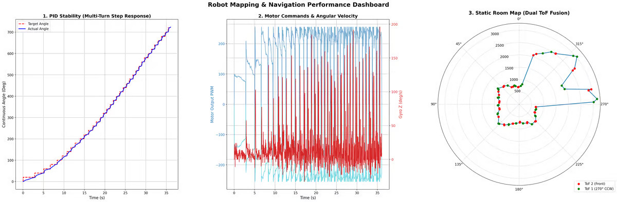
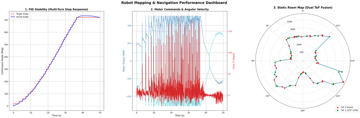
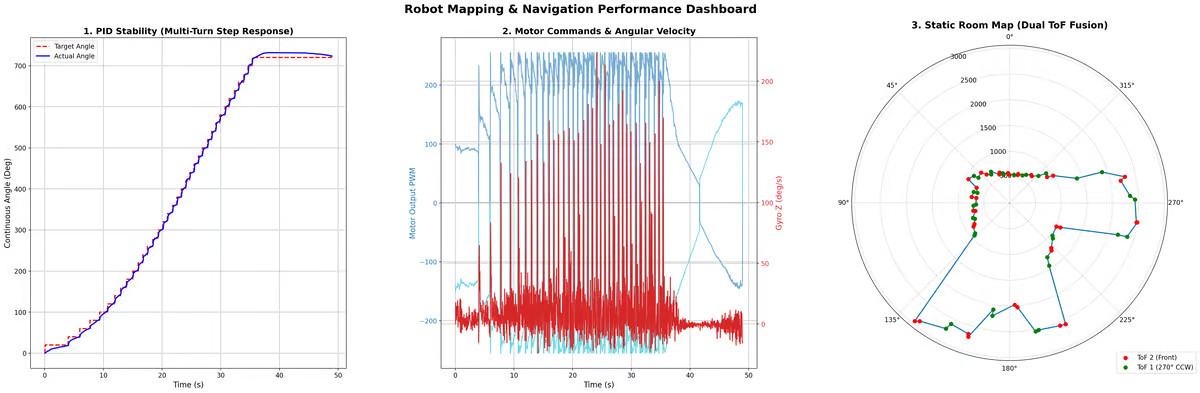
I executed the mapping turn at five marked positions in the lab space: (0,0), (-3,-2), (5,3), (0,3), and (5,-3). At each location, I used two ToF sensors while the robot performed a 720° or 1080° rotation, corresponding to roughly 20° angular increments. This produced approximately 36 or 48 samples per sensor, or about 72 to 96 total measurement points per location after combining both sensors.

Video Here

I defined the robot frame to be aligned with the world frame, so there was no initial rotation or translation offset between them. In my coordinate convention, 0° points toward the positive y-axis and 90° points toward the positive x-axis. So for all five scans, I started the robot facing the positive y-direction. This made it easier to directly interpret the yaw angle and convert the measured distances into the global frame.

Readings at (-3,-2)

Readings at (0,0)

Readings at (0,3)

Readings at (5,3)

Readings at (5,-3)

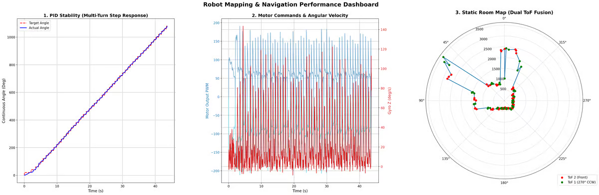
The polar coordinate plots from the five scan positions match the expected room geometry well. The two ToF sensors produce consistent and complementary measurements, and their combined data forms a coherent outline of the surrounding environment. In addition, scans collected over different numbers of rotations produce similar wall shapes, indicating that the angular step control is repeatable and that the measurements are reasonably stable across repeated turns.

Final Map

After transforming all measurements from the five scan locations into the global frame, I combined the resulting point clouds into a single map.

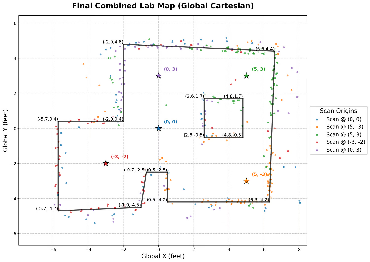
The merged scatter plot captures the overall geometry of the room well.

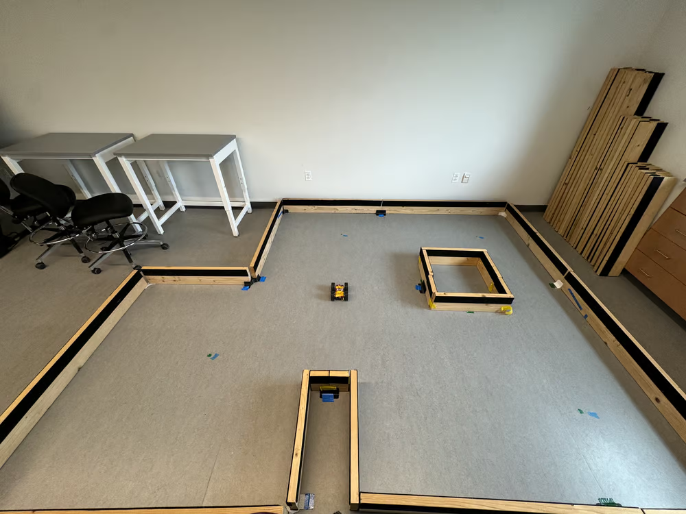
Although there are some slight errors in the merged result, such as small wall slopes or local misalignment, the overall pattern matches the true lab space closely.

To convert the map into a format usable by the simulator, I manually estimated the wall and obstacle boundaries from the merged scatter plot and represented them as a set of line segments. Each line is stored by its start and end points, $(x_{start}, y_{start})$ and $(x_{end}, y_{end})$.

ground_truth_lines = [
    [(-5.9,0.6), (-5.9, -4.7)], # External Walls 
    [(-5.9,0.6), (-2.2, 0.6)],
    [(-2.2,4.8), (-2.2, 0.6)],
    [(-2.2,4.8), (6.8, 4.5)],
    [(6.8,4.5), (6.4, -4.3)],
    [(0.3,-4.3), (6.4, -4.3)],
    [(0.3,-4.3), (0.3, -2.5)],
    [(-0.7, -2.5), (0.3, -2.5)],
    [(-0.7, -2.5), (-0.8, -4.5)],
    [(-5.9, -4.7), (-0.8, -4.5)],
    [(2.7,1.6), (4.8, 1.6)],  # Internal Walls 
    [(2.7,1.6), (2.7, -0.5)],
    [(2.7, -0.5), (4.8, -0.5)],
    [(4.8, -0.5), (4.8, 1.6)]
]